Section 11.3 Titles, Labels, and Legends

The plots that we have created so far looked good, but they lack the information necessary to make them good plots. Namely, they need axes labels, titles, and legends. Don’t worry! The hardest part of this chapter is done (looking at you SUBPLOT).

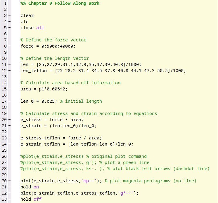
For now, comment out all of the stuff you have about subplots. We are going to concentrate on the plot with the HDPE and Teflon data on the same axes. If you have been following along, you should have something very similar to figure 11.3.1 below. We are going to start at line 34, just below all this stuff.

When you hit run on the script above, you should get a figure with magenta pentagrams connected by a dotted line and green stars connected by a dotted line on the same axes. Note that the magenta stars are the HDPE data and the green stars are the Teflon data.

Adding a Title

To add a title to the plot, use the title() function. That is it. The title function accepts a character string input. So if we wanted to create a title for the plot called “Tensile Test Data” we would add a new line to our script that looks like this:

title('Tensile Test Data');

Go ahead and add that line to your script and re-run it. I told you it was easy! Just remember that the input to the title() function must be a character string which just means it needs ' marks surrounding the text.

Adding Axes Labels

To add axes labels to the plot, we are going to use the xlabel() and ylabel() functions that correspond to the x-axis and y-axis respectively. Just like with the title() function we need to input the character string. Since in this particular plot the x-axis corresponds to the strain which is unitless and the y-axis corresponds to stress which has units of Pascals, we just need to add the following two lines of code:

xlabel('Strain (ratio)');

ylabel('Stress (Pa)');

Add those lines, re-run the script and watch the magic happen!

Adding a Legend

MATLAB makes creating legends easy, but you have to remember the order in which you plotted your data. In this example, we plotted the HDPE data before the Teflon data. So to add an appropriate legend we would use the legend() command, and then supply character string inputs that correspond to the data. For example:

legend('HDPE','Teflon');

Notice that when you add that line to your script and re-run it, you get a nice little legend! Nifty huh? There are some more advanced functionalities to the legend() function that won’t be discussed in this book. But if you are interested type in help legend and check out some of the other features!

The Final Script

If you have been following along, this is what your final script should look like. Keep in mind the subplot stuff is commented out below. If I were you, I wouldn’t delete it!