Section 11.4 Plotting Functions

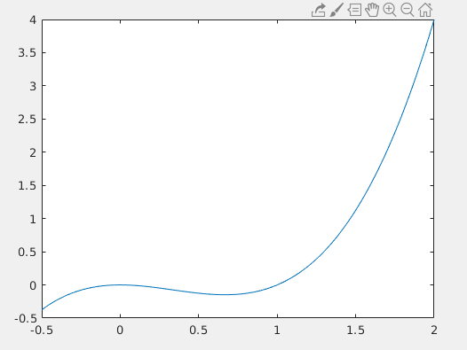
Once you have mastered plotting in MATLAB plotting functions is actually very easy. For example, lets make a simple plot of \(y=x^3-x^2\) from \(x=0.5\) to \(x=2\text{.}\)

In the previous chapter, there was an example that showed us how to evaluate a function at different values. The key was to first, create an array of ( x ) values, then mathematically evaluate those ( x ) values with the mathematical function of interest. We will do the same thing here. In your script, type:

x = -0.5:0.01:2;

y = x.^3 - x.^2;

Notes: We choose an increment of 0.01 so that the graph looks “smooth”. What we are really doing is creating a non-smooth graph but since the increment is so small, it appears smooth. Also, remember, we need the .^ because we are performing exponentiation on the ( x ) array.

Now, lets plot ( x ) versus ( y ).

You should see a graph pop up that looks like figure 11.4.2. That’s all there is to it!