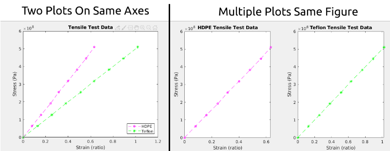
A lot of the time it is useful to show someone multiple plots. Perhaps you want to compare two materials or show different projections. MATLAB has the capability to plot multiple plots on the same axes or display multiple plots in the same figure. See figure 12.2.1 below for an example.
You should have also noticed that the plots in Figure 12.2.1 above have titles, axes labels, and legends (where appropriate). In the next section of this chapter, we will learn how to accomplish this. For now, let’s concentrate on what we need to learn to do either:
Before we jump into learning those two points, you should have noticed that I added tensile testing data on Teflon to the charts. To follow along, you will need to do so as well. Go ahead and add a new array called \(len_teflon\) to your script with the following values:
We will consider the case where the Teflon specimen has the exact same starting dimensions as the HDPE specimen we are using before. We will also test the Teflon under the exact same engineering stresses. With that being said, calculate the engineering stress in an array called e_stress_teflon and the engineering strain in an array called e_strain_teflon. Do not skip ahead to see my solution UNTIL you have tried it yourself!
Now that we have two sets of data, we can practice plotting them on the same axes. To do so, you just need to pretend you are a cowboy, and that MATLAB is a horse. So we just need to tell MATLAB “to hold on there partner, I want to plot multiple plots on the same axes”.
I wasn’t kidding! You really just have to add the line hold on to your script! For example, if we wanted to plot the HDPE and Teflon tensile test data on the same axes, we can just type in:
Here is an interactive code box that functions similarly to the MATLAB command window. Note that this web version does NOT support graphics so you’ll need to copy this code into your MATLAB window!
The first line plots the HDPE data as we have done before (make sure you know what 'mp--' does!). The second line (hold on) tells MATLAB to wait and plot subsequent plots on the same axes. After you turn hold on, MATLAB will put ALL plots on those axes. Therefore, it is a good idea to turn hold off when you are done in case you need to plot other things, not on the same axes.
In this particular example (tensile test data of HDPE and Teflon) it makes the most sense to plot the graphs on the same axes. But for the sake of learning, let’s go ahead and create a new figure window and create multiple plots in the same figure window. To do so, we will need to use the subplot() function.
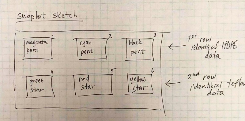
Then think about how you want your plots arranged. It really helps to sketch it out on a little piece of paper (kind of like in figure 12.2.5) to get a good idea. Let’s say for this example we want 2 rows and 3 columns of plots.
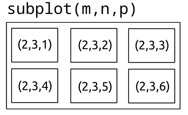
The subplot(m,n,p) function divides the figure window into mxn rectangular plots. The p indicates the number of the subplot. The subplots are numbered starting at 1 in the upper left corner and increasing in number from left to right. Figure 12.2.5 is illustrating this. For the plot in the upper left corner, the user would type in:
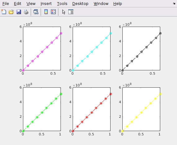
Go ahead and try creating a 2x3 subplot grid with our tensile test data. You can reuse the data, so this IS a contrived example after all! But it is good practice.
I suggest sketching out your plan. Change the colors between each subplot and write them out on paper BEFORE you code to make sure you understand what is going to happen.
It is ok to struggle a little bit here! Don’t jump straight to the solution until you try it! Subplots are kind of complicated and not straightforward but you need to practice.
Correct. A 2-by-3 subplot layout has 2 rows and 3 columns. MATLAB numbers the subplots from left to right, top to bottom, making the subplot in the 3rd column of the 2nd row position 6.
subplot(3,2,6)
Incorrect. This creates a 3-by-2 subplot layout rather than a 2-by-3 layout.
subplot(6,2,3)
Incorrect. The first two arguments specify the number of rows and columns, not the total number of subplots and columns.
Here is an interactive code box that functions similarly to the MATLAB command window. Note that this web version does NOT support graphics so you’ll need to copy this code into your MATLAB window!