There is actually one more important way that we can use relational operators, we can use them in combination with mathematical operators. For example, we COULD perform an operation like this.
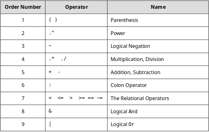
The problem is that we have not discussed the order of precedence (link is to MATLAB’s description). This is very similar to the mathematical concept of the order of operations. The only difference is that the order of operations does not include the relational or logical operators (we will talk about them later). Just like the order of operations, the order of precedence lets us know what mathematical, relational, and logical operation steps will happen in what order. MATLAB’s order of precedence is presented in figure 13.3.3 below.
You can think about it like the operators are waiting in line to get into a club. The bouncer is going to let everyone in but they don’t all get to come in first come first serve. There is a hierarchy, and that hierarchy is listed in table 13.3.3 below.
You should note that this is slightly different than what MATLAB presents as the order of precedence, I truncated the official list down to what we will be using in this book. Let’s take another look at that MATLAB statement we started this section with:
Now we can see how to apply the order of precedence and evaluate this statement! The best way to solve these types of statements is to reduce according to the order of precedence and then continue. For example:
Now our statement has reduced to: pie + 3136 > tomato * salmon + 2 Next on the order of precedence is .*. We have one multiplication operation, tomato * salmon = \(23*56=1288\text{.}\)
Now our statement has reduced to: pie + 3136 > 1288 + 2 We now perform the math operations. Recall pie = pi*2 which is \(\approx 6.2832\text{.}\) So… pie + 3136 = \(6.2832+3136=314.2832\) and 1288 + 2 = \(1230\)