Section 5.4 Formulas (\(=\)) and Cell Referencing
Now that we are familiar with cell addressing and how to enter data into cells, we can begin to explore one of the most powerful features of Excel, using cell formulas.
By using formulas, we can have Excel perform a calculation and show the result in the cell that contains the formula. Excel formulas start with an
= sign and work essentially like a calculator. For example, if we wanted to calculate the area of a circle (recall \(area=\pi*r^2\)), with a radius of 0.24 meters, we could simply type the following formula into any cell (let \(\pi\) be approximated by 3.1415).
= 3.1415 * 0.24^2
Voila! We can then see that the area is \(0.18095\,meters^2\text{.}\) However, we are missing the true power of Excel in this case which is cell referencing.
To see an example of cell referencing in action, let’s consider a situation where we need to calculate the areas of a bunch of different circles. To start, recreate the spreadsheet shown in Figure 5.4.1 (you should be able to recreate this using the formatting tools highlighted in Figure 5.3.3).
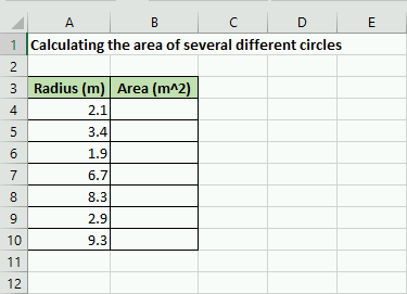
So now all we need to do is tell Excel to calculate those values and store the corresponding area in the appropriate B cell. To do that, we could just type in an individual formula into each appropriate cell.
For example, you could (but you shouldn’t) type the following into
B4:
3.1415 * 2.1^2
Then we could (again, don’t do this) type the following into
B5:
3.1415 * 3.4^2
But you can already see this would be exceptionally tedious! Especially if we wanted to calculate hundreds or even thousands of areas! This is where cell referencing comes into play. The key is to notice that the value
2.1 is stored in cell A4. The power of Excel is that we can actually just reference the cell A4 in the formula.
You should type the following into cell
A4:
3.1415 * A4^2
Once you hit enter, you can see that it uses the data from the cell
A4 in the calculation. Now, here is the trick. You can use cell addressing to create formulas and calculate the areas for the other cells automatically! To do so, select cell B4 by clicking on it. You should notice a little green box (called the “fill handle”) in the lower right corner. Click on that, and drag it down so that it fills all the cells in which we would like to calculate an area. This is called copying the cell formula. If you are a little confused about what to do, see Figure 5.4.2 below.
What you should notice (and can see in Figure 5.4.2 in the link above) is that Excel automatically creates new formulas that have the correct cell address! That is because when we copied the formulas to the new cells Excel assumed that we wanted it to create a new formula with a cell in the same relative position as
A4.
For example, let’s think about the new formula in
B10. You can see the new formula by double-clicking on it. Notice that the new formula is:
= 3.1415 * A10^2
Since
B4 (the location of the original formula) is 6 cells above B10, when we copied the formula, Excel automatically adjusted the A4 from the original formula to A10 because it is 6 cells lower. That is called relative cell addressing. There are two more types of cell addressing in Excel.
For instance, lets say that instead of typing 3.1415 we wanted to store an approximation of \(\pi \approx \frac{22}{7}\) into a cell and use that in our calculations. To do so, add
=22/7 to the cell D4 and format it like the figure below.
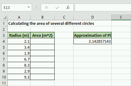
Hopefully, you can see that relative cell addressing will be a problem in this case. To see what I mean, type
=D4*A4^2 into cell B4. Everything should be ok. But when you try to copy the formula down to B10 you should notice that everything is filled with 0. What is going on? If you look at one of the formulas (for example see the new formula in cell B6), you should notice that instead of cell D4 which corresponds to our approximation of \(\pi\text{,}\) Excel assumed we wanted to try and use a value in D6 for the calculation. Since there is nothing in D6, the calculation is equal to 0!
What we need to do to fix it, is go back to the formula in
B4 and create an absolute cell address for D4. To do so, add $ symbols in front of both the D and the 4 like this: $D$4. Now when you try to copy the formula to the cells below, it will use relative cell addressing for the A cells (which is what we want) and it will use absolute cell addressing for the D4 cell! A short video showing this is in the figure below.
The last little piece when it comes to cell addressing is there is one more form Excel accepts, mixed addressing. You can fix either the row or the column designation by adding a
$ sign. For example, D$4 would only fix the row and would allow the column to change if the formula is copied.
To recap this section, there are three types of cell addressing that you can use in your Excel formulas:
-
Absolute Addressing: in this case, Excel will always refer to the exact same cell if the formula is copied to a new location. You create an absolute cell address by adding a
$immediately before both the column and row of the cell of interest (e.g.$B$5) -
Relative Addressing: in this case, Excel will refer to the cell in the same relative position as the cell containing the formula, no matter where the formula is copied in the worksheet. (e.g.
B5) -
Mixed Addressing: in this case, either the row or the column is fixed. (e.g.
$B5)

