Section 8.5 Exponential Models
Exponential models are also swoopy (and hence the reason you need to think to make sure you don’t confuse it for a power model!) and take on the form of the equation:
\(y=be^{mx}\)
Keep in mind that the \(e\) in this equation refers to the mathematical constant, the base of the natural logarithm. There are a couple of other interesting things to note about exponential models:
-
The value \(b\)is the value at the start of the exponential growth (or decay).
-
The \(m\) is called the rate of growth.
-
When \(m\) is positive, the model is asymptotic to 0 for large negative values of \(x\text{.}\) This scenario is called exponential growth.
-
Conversely, when \(m\) is negative, the model is asymptotic to 0 at large positive values of \(x\text{.}\) This scenario is called exponential decay.
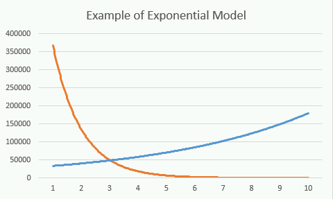
Example of an Exponential Model- Atmospheric Pressure

The “standard” pressure at sea level is 101,325 Pascals. The reason standard is in quotes is because realistically it varies with the weather, temperature, etc. but that is the number scientists commonly use to calculate things. Furthermore, it is known that atmospheric pressure, if you could provide existing plans, decreases by about 12% for every 1,000 meters that you go up. Intuitively, you can see that this is an example of exponential decay! Furthermore, with a little cleverness, we can create a mathematical model and guess what the pressure should be in Fort Collins, CO (elevation 5,003 feet) and on the top of Mount Elbert, the highest peak in Colorado (elevation 14,439 feet or 4,041 meters).
The elevation of Fort Collins is listed at 5,003 feet. Take a minute to take out a piece of paper, look at your conversion sheet, and convert this elevation to meters. This is a good brain workout review! Don’t skip it!
Looking at our model:
-
We know that \(b=101325\) because that is the pressure at sea level in Pa and the \(b\) is the value of what we are modeling before the decay.
-
We know \(y\) is our pressure in Pascals and \(x\) is the distance above sea level in meters.
-
We know that at \(x=1000\text{,}\) \(y\) is \(12\)% less than at sea level. We can use this to figure out what \(m\) is equal to!
\(12\)% of \(101325\) is \(12,159\text{.}\) That means that \(y(1000)=1010325-12159=89166\text{.}\) This implies that the pressure at 1000 meters is 89,166 Pascals. Make sure you can follow this logic!
Plugging in everything we know to solve \(m\text{:}\)
\(89166=101325e^{1000m}\)
Solving for \(m\text{:}\)
\(m=\frac{ln(0.88)}{1000}\)
Now our mathematical model becomes:
\(y=101325e^{\frac{ln(0.88)}{1000}x}\)
and we can use this to calculate the expected atmospheric pressure on the top of Mount Elbert!
Atmospheric Pressure on the top of Mount Elbert
\(x=4401\) \(y==101325e^{\frac{ln(0.88)}{1000}4401}=57727\,Pa\)
You can validate for yourself with a quick google search that this is a pretty accurate model!
Using the mathematical model we just developed for atmospheric pressure, what is the predicted atmospheric pressure in Fort Collins, Colorado?

