Obesity has become a widespread health concern, especially in children. Researchers believe that giving children easy access to food increases their likelihood of consuming extra calories.
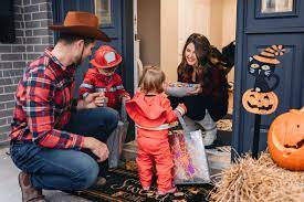
Schwartz, Chen, and Brownell (2003) examined whether children would be willing to take a small toy instead of candy when trick-or-treating on Halloween. They had seven homes in 5 different towns in Connecticut present children with a plate of 4 toys (stretch pumpkin men, large glow-in-the-dark insects, Halloween theme stickers, and Halloween theme pencils) and a plate of 4 different name brand candies (lollipops, fruit-flavored chewy candies, fruit-flavored crunchy wafers, and "sweet and tart" hard candies) to see whether children were more likely to choose the candy or the toy. The houses alternated whether the toys were on the left or on the right. Data were recorded for 284 children between the ages of 3 and 14 (who did not ask for both types of treats).
The parameter of interest is the probability (or long-run proportion) that a child, when presented with a choice between toys and candy while trick-or-treating, will choose the toy.
State an appropriate null and alternative hypothesis involving this parameter (in symbols and in words), for testing whether there is strong evidence of a preference for either the toys or the candy.
What does "theory" predict for the mean and standard deviation of the distribution of "number of successes" under the null hypothesis if we model this experiment as a binomial process? Do you expect this distribution to be symmetric and "filled in" or skewed and "gappy"?
The normal distribution has many, many applications to quantitative variables in general (e.g., many biological variables like height are assumed to follow a normal distribution). For now, we will focus on using this mathematical model as an approximation to the null distribution.
If the sample size is large enough, then the distribution of "number of successes" for a binomial random variable will be well-modeled by the normal probability distribution. The sample size is considered large enough if \(n\times\pi\geq 10\) and \(n\times(1-\pi)\geq 10\text{.}\)
When \(\pi\) is close to 0 or 1, the binomial distribution becomes more skewed. We need both \(n\pi\) and \(n(1-\pi)\) to be large enough to ensure the distribution is symmetric enough to be well-approximated by a normal distribution. If \(\pi\) is very small, even with a large \(n\text{,}\) we might not have enough expected successes for the normal approximation to work well.
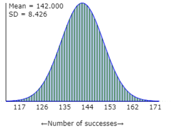
The mean is at 142 and the standard deviation is at 8.43. The normal distribution overlay matches up pretty well with the binomial distribution though we do see some spaces between the bars.
There are actually some nice advantages to using the normal distribution rather than the binomial distribution, though less so as computers have become so advanced. For one, tail probabilities can be approximated by finding the area under the normal curve rather than summing binomial probabilities.
In the sample, 135 children chose the toy and 149 chose the candy. Use the applet to find the following two-sided p-values, and explain briefly how each is found:
Simulation: Approximately 0.40 (will vary) - found by simulating many samples from a binomial distribution and counting the proportion as extreme or more extreme than 135.
When switching to proportions, the null distribution is centered at \(\pi = 0.5\) instead of 142, and the standard deviation becomes \(\sqrt{\pi(1-\pi)/n} = \sqrt{0.5(0.5)/284} \approx 0.0297\) instead of 8.43.
When the Central Limit Theorem applies, the distribution of sample proportions is approximately normal with mean equal to \(\pi\) and standard deviation equal to \(SD(\hat{p}) = \sqrt{\pi(1-\pi)/n}\text{.}\)
When we are using the normal distribution, it is even more common to work with the "standardized statistic" by calculating how many standard deviations the statistic is from the expected value (mean) of the null distribution.
Standardize the value of the statistic for the Halloween study by comparing to the mean and standard deviation of the distribution of sample proportions. Interpret your result in context.
Interpretation: The observed sample proportion of 0.475 is 0.84 standard deviations below the expected value of 0.5 under the null hypothesis. This is not particularly unusual.
The "zero" subscript indicates that this is the value calculated under the null hypothesis (using \(\pi_0\text{,}\) the hypothesized value of the parameter).
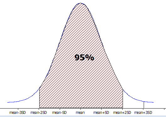
In any normal distribution with mean \(\mu\) and standard deviation \(\sigma\text{,}\) we expect the interval \((\mu - 2\sigma, \mu + 2\sigma)\) to capture approximately 95% of the distribution. In other words, 95% of sample proportions should fall within \(2 \times \sqrt{\pi(1-\pi)/n}\) of \(\pi\text{.}\) So with a normal distribution, the two-standard deviation guideline matches up with a two-sided p-value below 0.05.
Since \(|z| = 0.84 < 2\text{,}\) the observed result is within 2 standard deviations of the expected value under the null hypothesis. This suggests the null hypothesis is plausible - we do not have strong evidence against it. The p-value should be greater than 0.05.
Use technology to find the corresponding p-value. [Hints: You can calculate the probability from the z-value using standard normal distribution (mean 0, SD 1), e.g., Normal Probability Calculator applet; or use the Technology Detour below to carry out a one-sample z-test.]
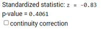
Using technology (Normal Probability Calculator or z-test function), the p-value is approximately 0.40 (or 0.401). This confirms our conclusion that the result is not statistically significant.
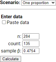
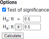
For the Halloween study, enter \(n\) = 284 and either 135 successes or 0.475 as the proportion. Set the hypothesized value to 0.5 and select a two-sided alternative.
If children were equally likely to choose toys or candy, we would observe a result as extreme as or more extreme than 135 out of 284 children choosing toys in about 40% of samples.
Do you think the researchers are pleased by the lack of significance in this test? Explain, in the context of the study, why such a result might be good news for them.
Yes, the researchers should be pleased! The lack of significance means there’s no strong evidence that children prefer candy over toys. This is good news because it suggests that offering toys as an alternative to candy is viable - children are willing to accept toys instead of candy. If there had been strong evidence of a preference for candy, it would suggest that offering toys wouldn’t be an effective strategy to reduce candy consumption.
Even though we passed the "validity conditions" for the normal approximation for this study, we could still use a "continuity correction" to improve the approximation.
The exact binomial p-value should be closer to the simulated p-value. This is expected because the simulation approximates the true binomial distribution, while the normal approximation is just that - an approximation to the binomial.
In the binomial distribution \(P(X = 135) = 0.220\text{.}\) What is \(P(X = 135)\) with the normal distribution? How do \(P(X < 135)\) and \(P(X \leq 135)\) compare in each distribution?
To make the normal probability (which is finding \(P(X < 135)\) closer to the binomial probability, which finds \(P(X \leq 135) = P(X < 135) + P(X = 135)\text{,}\) we want to include more of the area under the normal curve above 135 in our calculation. A continuity correction does this by using the normal distribution to find \(P(X < 135.5)\) instead. This does not change the binomial probability but should enlarge the normal probability.
In the One Proportion Inference applet, specify 135.5 in the As Extreme As box (if using number of successes as the statistic, otherwise use \(135.5/284 \approx 0.477\) instead) and press Count.
The applet uses 148.5 for the right-side cut-off. This is because 135.5 is 6.5 below the mean of 142, so by symmetry, we need 6.5 above the mean: \(142 + 6.5 = 148.5\text{.}\)
The p-value should increase slightly (become closer to 0.40) and should now be more similar to the exact binomial p-value. The continuity correction improves the normal approximation by accounting for the fact that the normal distribution is continuous while the binomial is discrete.
Many software programs allow you to apply this continuity correction for a one-sample z-test (e.g., using \(\hat{p} = (X \pm 0.5)/n\) as the input) or may do so by default. However, when n is large, you may not see much difference in the values.
For the Halloween study, after entering the data (\(n\) = 284, 135 successes), check the continuity correction box and observe how the p-value changes.
If we define \(\pi\) to be the probability that, when presented with a choice of candy or a toy while trick-or-treating, a child chooses the toy, and if we assume the null hypothesis (\(H_0\!:\pi = 0.5\)) is true, the above calculations tell us that we would observe at most 135 children choosing a toy or at least 149 of the 284 children choosing a toy (or at least 149 choose candy or at most 135 choose candy) in about 40% of all possible samples from such a process. Thus, this is not a surprising outcome when \(\pi = 0.5\text{.}\) We fail to reject the null hypothesis and conclude that it’s plausible that children are equally likely to choose the toy or the candy.
We do have some cautions with this study as it was conducted in only a few households in Connecticut, a "convenience sample," so we cannot claim that these results are representative of children in other neighborhoods. We also don’t know if the children found the toys "novel" and whether their preference for toys could decrease as the novelty wears off (or if "better" candy choices were offered). Furthermore, when the children approached the door they were asked their age and gender, and for a description of their Halloween costume. The researchers caution that this may have cued the children that their behavior was being observed (even though their responses were recorded by another research member who was out of sight) or that they should behave a certain way. Still, these researchers were optimistic that alternatives could be presented to children, even at Halloween, to lessen their exposure to large amounts of candy.
Dr. Güntürkün found 80 out of 124 couples leaned right in his sample. Find the one-proportion z-test statistic and normal-based two-sided p-value. Do the standardized statistic and p-value agree? How does the normal-based p-value compare to the exact binomial p-value for this study?
A student wanted to assess whether her dog Muffin tends to chase her blue ball and her red ball equally often when they are rolled at the same time. The student rolled both balls a total of 96 times, each time keeping track of which ball Muffin chased. The student found that Muffin chased the blue ball 52 times and the red ball 44 times. Let’s treat the blue ball as "success."
Suppose you want to redo this study using a sample size of 200 tosses. You plan to use a significance level of \(\alpha\) = 0.05, and you are concerned about the power of your test when \(\pi\) = 0.60. Calculate this power and interpret what “power” implies in this context.