The 1991 World Almanac and Book of Facts contained a section on “noted personalities” in a total of nine occupational categories. The lifetimes of these people can be found in the lifetimesFull.txt data file. Analyze these data to address the question of whether the average lifetimes across these occupational categories differ significantly. Include graphical and numerical summaries as well as a test of significance. Summarize your conclusions.
Solution.
To compare several groups on a quantitative variable, we will consider analysis of variance. The first step will be to describe the data we have. The file
lifetimesFull contains the lifetimes (years) of notable personalities from nine different occupation classifications. The samples were selected independently from within each job classification but they were presumably not selected at random. Thus, we should be cautious in how we generalize our conclusions. We will need to restrict our conclusions to “notable personalities” but otherwise might not suspect any bias in the World Almanac’s sampling method. In this case, we can define \(\mu_i\) to be the population mean lifetime for all notable personalities with occupation \(i\text{.}\)
\(H_0\!:\) \(\mu_{scientist} = \mu_{writers} = \mu_{politicians} = \mu_{military} = \mu_{artists} = \mu_{philos} = \mu_{social} = \mu_{historians} = \mu_{business}\)
\(H_a\!:\) at least one population mean lifetime differs from the rest
Numerical and graphical summaries do reveal some differences across the groups.
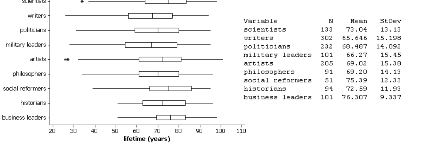
Side-by-side boxplots of lifetime (years) for the nine occupation groups, next to summary statistics: scientists n=133 mean 73.04 SD 13.13; writers n=302 mean 65.646 SD 15.198; politicians n=232 mean 68.487 SD 14.092; military leaders n=101 mean 66.27 SD 15.45; artists n=205 mean 69.02 SD 15.38; philosophers n=91 mean 69.20 SD 14.13; social reformers n=51 mean 75.39 SD 12.33; historians n=94 mean 72.59 SD 11.93; business leaders n=101 mean 76.307 SD 9.337.
There is a slight tendency for longer lifetimes among scientists and business leaders and for shorter lifetimes among writers and military leaders. However, there is a fair bit of variation within the groups and much overlap in the boxplots.
To decide whether an ANOVA procedure is valid, we check the technical conditions:
-
Dotplots of the individual samples do not reveal any marked departures from normality.
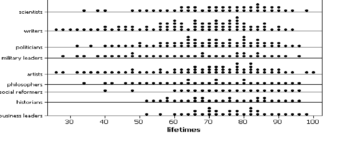
Stacked dotplots of lifetimes for the nine occupation groups, each roughly symmetric to slightly left-skewed with no marked departures from normality.
-
The ratio of the largest to smallest standard deviations (15.45/9.34) is less than 2 so we will assume that the population variances are equal.
-
We have independent samples from each population though the randomness condition is questionable.
Although we do not have randomness in this study, we will still explore whether the difference between the sample means is larger than we would expect by chance.
R
> summary(aov(lifetime~occupation))
              Df Sum Sq Mean Sq F value   Pr(>F)
occupation     8  14837  1854.6   9.359 1.26e-12 ***
Residuals   1301 257818   198.2
JMP
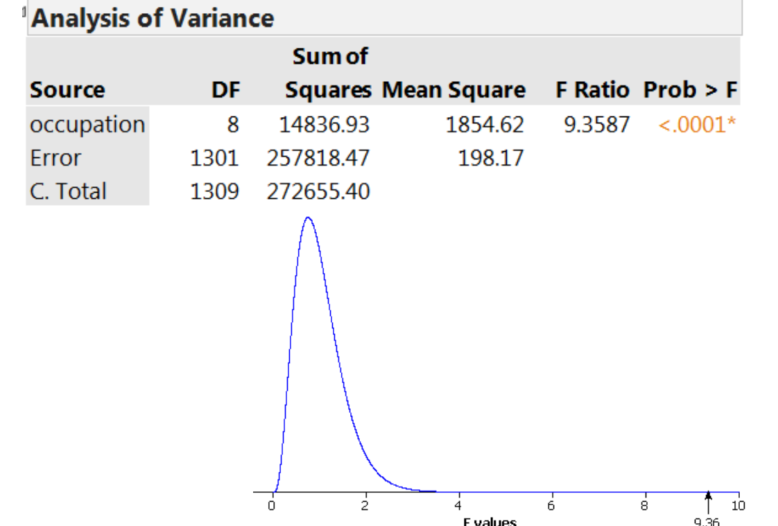
JMP Analysis of Variance table: occupation DF 8, Sum of Squares 14836.93, Mean Square 1854.62, F Ratio 9.3587, Prob greater than F less than .0001; Error DF 1301, Sum of Squares 257818.47, Mean Square 198.17; C. Total DF 1309, Sum of Squares 272655.40; below, an F distribution curve with the observed value 9.36 marked far in the right tail.
The large test statistic \(F = 9.36\) and small p-value (\(0.000 \lt 0.001\)) provide strong evidence that the population mean lifetime for at least one of these occupations differs from the rest.
Because this was an observational study, we cannot draw any cause and effect conclusions and as discussed above we should be cautious in generalizing these conclusions beyond the 1310 individuals in the study as they were not randomly selected. For the individuals in this study, there appears to be something other than random chance to account for the differences we observed in their lifetimes.

