Previous research has demonstrated that domesticated dogs can be trained to understand human cues, such as looking or pointing at an object. But it was not clear how the animals would perform with "behavioral cues" showing intent such as reaching for, but not obtaining, or trying to open an object.
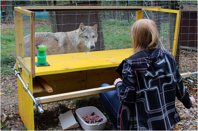
Lampe et al. (2017) gave captive wolves, pack dogs living in identical conditions to the wolves, and pet dogs living with families a series of "object-choice tasks." A table was placed outside a fenced compartment, and a container was placed at each end of the table, one containing food and one empty. The experimenter would give the cue as to which container had the food and then the animal would touch one of the two targets next to the containers. A 6-year-old female timber wolf, Yukon, chose the intended container in 6 of the 8 trials with behavioral cues.
In drawing conclusions beyond our sample data to the underlying random process, we will often be choosing between two competing claims about the underlying process:
In Investigation 1.1, the null hypothesis was that infants (in general) choose equally among the two toys in the long run. The alternative hypothesis was that infants have a genuine preference for the helper toy.
So our simulation model is going to assume the null hypothesis is true and we will see how unusual it is to find 6 successes and 2 failures in 8 attempts. Can we use "coin tossing" again? How many times will we toss the coin?
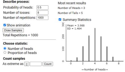
Yes, we can use coin tosses again with heads = Yukon correct and tails = Yukon incorrect. We want to use 8 tosses for each repetition and count how many heads we have.
Use the One Proportion Inference applet to carry out 1,000 repetitions of the simulation. Check the Summary Statistics box and report the mean and standard deviation of your simulated distribution of "could have been" outcomes.
Based on your simulation results, which assumes Yukon is guessing, should we be very surprised to see 6 correct guesses? Explain/support your reasoning.
An outcome of 6 heads does not appear to be in the tail of the distribution and so does not appear to be an unusual outcome when the null hypothesis is true.
In Investigation 1.1, the observed result (14) was pretty far in the tail of the distribution and you probably agreed that we could consider it unusual. This result (6 out of 8) is not as inconsistent with the null hypothesis; so where do we "draw the line"? First, we need to agree on a measure of "rareness." We could just calculate the theoretical probability of 6 heads in 8 tosses (0.1094), but keep in mind that if we have a larger sample size (e.g., 100 tosses), then any individual outcome (e.g., 62 heads) will have a small probability. So we want to judge how extreme our observation is relative to the other observations in the simulated distribution. One way to do this is to count how many outcomes are as or even more extreme (even further from the expected value) than the observed outcome. For example, if we tell you that only 1% of rattlesnakes are longer than 2.5 meters, then you know to be very surprised to see a 3-meter rattlesnake and you may even begin to think that what you are looking at is not a rattlesnake at all!
In 1,000 repetitions, assuming the probability of choosing correctly is 0.50, we found % of repetitions of 8 attempts to result in 6 or more successes.
Because the simulation assumes the null hypothesis to be true, we can refer to the distribution you simulated as the null distribution. When you determine the proportion of the results in the null distribution that are at least as extreme as the observed result, you are estimating a probability. We will refer to this probability as the p-value. We use the p-value to evaluate the strength of evidence against the null hypothesis.
The smaller the p-value, the stronger the evidence against the null hypothesis. There are no hard-and-fast cut-off values for gauging the smallness of a p-value, but generally speaking:
Because we are assuming a random process, we can use probability rules to calculate an "exact" value for the p-value. In fact, we have been assuming a very special random process, a binomial process.
Because we are assuming the null hypothesis to be true, we are treating each attempt as an identical repetition of a random process with a probability of success of 0.50 for each attempt (always two containers to choose from), and one attempt outcome does not impact the probability of success on the next attempt (e.g., a screen was lowered between attempts and the location of the food randomized each time) so the attempts are independent. We are counting \(X\text{,}\) the observed number of correct choices in the \(n = 8\) trials. So \(X \sim\) (is distributed as) \(\text{Binomial}(8, 0.50)\) and we want to determine the probability of observing 6 or more successes in 8 attempts by chance alone, \(P(X \geq 6)\text{.}\) We will illustrate this calculation next, and then turn to technology to find binomial probabilities.
Let S represent Success and F represent Failure. Consider one particular outcome for the 8 trials with 6 successes: SSFSSSFS. Because we are assuming the trials are independent, we can find the probability of this event by multiplying together the probabilities of the individual outcomes in the event.
But there are other possible outcomes that would also result in 6 successes and 2 failures (for example, SFSSSSSF). How many ways are there to arrange the 6 successes among the 8 slots?
This is where the binomial coefficient comes in handy. This binomial coefficient, denoted by \(C(n, k)\) or \(\binom{n}{k} = \frac{n!}{k!(n-k)!}\text{,}\) counts the number of ways there are to select \(k\) items from a set of \(n\) items. In this case, we want to find the number of ways to select 6 spots from the 8 trials for the successes:
Because the 28 outcomes corresponding to 6 successes are mutually exclusive (can’t occur simultaneously), we can find the probability of at least one of them happening by adding all of the probabilities together:
In general, the binomial probability of obtaining \(k\) successes in a sequence of \(n\) independent trials with success probability \(\pi\) on each trial is:
How does the binomial distribution match up to your earlier simulation results? How does the binomial (or “exact”) p-value compare to what you simulated earlier? Did everyone in class obtain the same “exact” p-value?
Write a one-sentence interpretation of this p-value in this context. Key components to include: what random process is being repeated, what is the null hypothesis that we are assuming to be true, what is the observed result we are considering, which outcomes are we considering to be more extreme?
If we were to repeatedly examine samples of 8 attempts from wolves who do not understand the communication cues, we would expect a about 15% of wolves to pick the correct container 6 or more timesby chance alone.
No, a p-value of 0.14 is not strong evidence against the null hypothesis. It is plausible that Yukon would do as well in 8 trials even if she didn’t understand the cue and was simply guessing.
If we assume Yukon is guessing between the two containers, regardless of the cue, then finding 6 or more successes in 8 trials is actually not very surprising (binomial p-value = 0.1445); about 14% of samples from a 50/50 process would show 6 or more successes in 8 trials. This does not provide convincing evidence that Yukon can perform "above chance," but there is not information about whether other wolves or other cues would show better performance.
lower.tail = TRUE if you want the probability less than or equal to the observed value, FALSE if you want the probability greater than or equal to the observed value
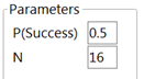
Using the Distribution Calculator in the ISCAM Journal File (download this file to your computer and then open the .jrn file to launch JMP). For the Friend or Foe study:
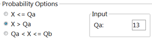
JMP Reminder: In JMP’s Distribution Calculator, you need to subtract 1 from your observed value when using the \(\geq\) option because JMP calculates \(P(X > Q_a)\) as \(P(X \geq Q_a + 1)\text{.}\) So to get \(P(X \geq 14)\text{,}\) you enter 13 as \(Q_a\text{.}\)
Use technology (R or JMP) to calculate the binomial p-value for the wolf study with 6 successes in 8 attempts, assuming \(H_0\!: \pi = 0.50\text{.}\) What binomial p-value do you obtain?
When Yukon was given "communicative cues" (looking at the container, pointing to the container) instead of behavioral cues, she was correct in 7 out of 8 attempts. Does this outcome provide convincing evidence that wolves understand communicative cues?
Across the 12 wolves in the study, in the 64 trials with communicative cues, the wolves understood the cue 41 times. What is the new p-value for these results? Explain why this would not be an appropriate analysis.
A study in Psychonomic Bulletin and Review (Lea, Thomas, Lamkin, & Bell, 2007) presented evidence that "people use facial prototypes when they encounter different names." Similar to one of the experiments they conducted, you will be asked to match photos of two faces to the names Tim and Bob. The researchers wrote that their participants "overwhelmingly agreed" on which face belonged to Tim. You will conduct a similar study in class to see whether your class also agrees with which face is Tim’s more than you would expect from random chance (here "random chance" = there is no facial prototyping and people pick a name for the face on the left at random).