Suppose we have data on the height (in centimeters) of boys for 3 different random samples at ages 2, 3, 4. The data in hypoHt.txt are modeled after data from the Berkeley Guidance Study which monitored the height (and weight) of boys and girls born in Berkeley, California between January 1928 and June 1929.
Do you expect the 2-year-old boys to all have the same height? Do you expect the 3-year-old boys to all have the same height? Do you expect the mean height of the 3-year-old boys to be the same as the mean height of the 2-year-old boys? Explain.
We expect there to be variability in the boys’ heights within ages but we also expect a tendency for the 3 year old boys to be taller than the 2 year old boys in general.
The regression equation for these sample data turns out to be \(\hat{height} = 75.2 + 6.47\,age\text{,}\) with a correlation coefficient of \(r = 0.857\text{.}\)
Is it possible that in the population of all Berkeley boys in the 1920s, there really is no linear relationship between age (2-4 years) and height, but that we obtained a correlation coefficient and sample slope coefficient this large just by random chance? Explain.
Describe how we might investigate the likelihood of obtaining such sample statistics by chance alone, if there really were no association between age and height in the population.
One way to determine whether our sample slope is significantly different from a conjectured value of the population slope is to assume a mathematical model.
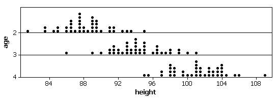
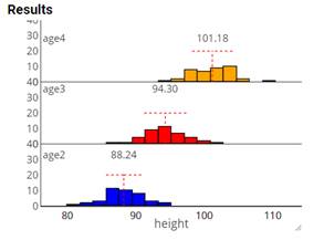
To understand the most basic regression model, consider conditioning your data set on a particular value of \(x\text{.}\) For example, let’s look at the distribution of heights for each age group.
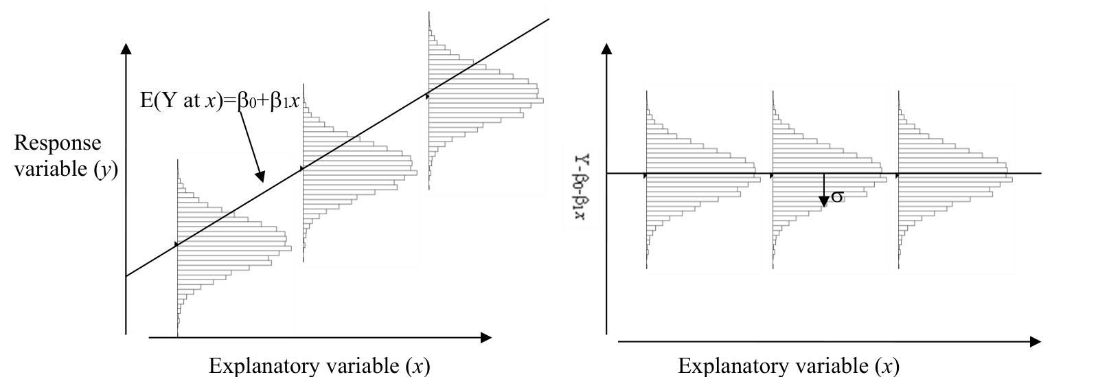
The relationship between the mean (expected value) of the response variable and the explanatory variable is linear: \(E(Y \text{ at each } x) = \beta_0 + \beta_1 x\text{.}\)
The variability of the observations at each value of \(x\text{,}\)\(SD(Y \text{ at each } x)\text{,}\) is constant. We will refer to this constant value as \(\sigma\text{.}\) This means that the variability of the (conditional) response variable distributions does not depend on \(x\text{.}\)
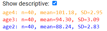
These conditions do appear to be met for the Berkeley boys’ heights. We have a normal distribution at each \(x\) and the spread of each distribution is similar.
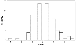
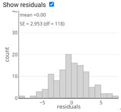
In the above example, checking the conditions was straight forward because we could easily examine the distribution of the heights at the 3 different values of \(x\text{.}\) When we don’t have many repeat values at each value of \(x\) we will need other ways to check these conditions. However, you should notice that the only thing that changes about the distribution of the response as we change \(x\) is the mean. So if we were to subtract the mean from each observation and pool these values together, then we should have one big distribution with mean 0, standard deviation equal to \(\sigma\text{,}\) and a normal shape.
Two diagrams. Left: a scatter of conditional distributions of the response variable at three values of the explanatory variable, each roughly normal, centered on the population regression line E(Y at x) = beta 0 plus beta 1 x. Right: the same three distributions after subtracting beta 0 plus beta 1 x, now all centered at a horizontal line at zero with common standard deviation sigma.
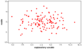
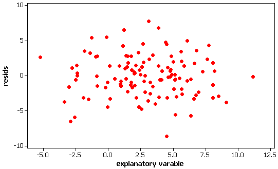
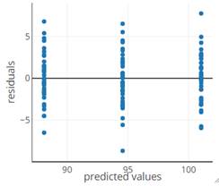
However we don’t know \(\beta_0\) and \(\beta_1\text{,}\) the population regression coefficients, but we have their least squares estimates. If we subtract the fitted values from each response value, these differences are simply the residuals from the least squares regression. So to check the technical conditions we will use residual plots.
The equal variance condition is considered met if a plot of the residuals vs. the explanatory variable shows similar variability in residuals across the values of \(x\text{.}\)
Another condition is that the observations are independent. We will usually appeal to the data being collected randomly or randomization being used. The main thing is to make sure there is not something like time dependence in the data.
The residuals plots show data that satisfy these conditions nicely, and in this case we would consider the \(t\)-procedures from Investigation 5.10 to be valid.