A group of students wanted to investigate which factors influence the price of a house (Koester, Davis, and Ross, 2003). They used http://www.househunt.com, limiting their search to single family homes in California. They collected a stratified sample by stratifying on three different regions in CA (northern, southern, and central), and then randomly selecting a sample from within each stratum. They decided to focus on homes that were less than 5000 square feet and sold for less than $1.5 million. The file housing.txt contains data for their final sample of 83 houses.
Copy and paste the url for housing.txt into the data window of the Analyzing Two Quantitative Variables applet (below) and press Use Data (twice), being sure to put price on the y-axis and squarefoot on the x-axis (use the Change variable selections pull-down menus) to create a scatterplot of the size vs. selling price for this sample.
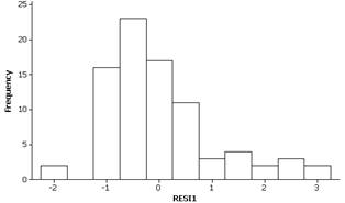
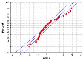
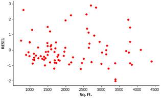
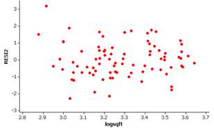
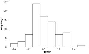
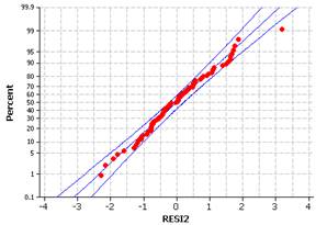
Check the Show residual plots box (under Explore models) in the applet to produce a histogram of the residuals (or a normal probability plot of the residuals), and a scatterplot of the residuals vs. the explanatory variable.
It takes a while to become comfortable interpreting these residual plots, but the housing data do appear to have some problems. The residuals appear to cluster closer to zero for the smaller houses and to have more variability for the larger houses. This violates the condition of a constant standard deviation for each value of \(x\text{.}\) There is also a very slight hint of some curvature in this graph. The distribution of the residuals is clearly non-normal. This residual analysis gives us several reasons to not apply the basic regression model to these data.
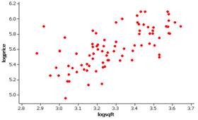
Check the log10 (log base ten) radio button for both the response variable and the explanatory variable. This will take the log base 10 of both the price and square footage variables. (If Show residual plots is still checked, the residual plots update to the transformed model.)
Examine the scatterplot of the transformed variables. Do these transformed variables appear to be more suitable for the basic regression model? Explain.
Although not perfect, these variables do appear to better follow the basic regression model. The residuals appear less skewed and there is less variation in the “width” of the residuals at different values of the explanatory variable. There does not appear to be any curvature in the relationship either.
If the log square footage increases by one (which corresponds to a ten-fold increase in square footage), we predicted the log price will increase by .890 (which corresponds to a \(10^{.89}\)-fold increase in price). If the log square footage is equal to 0 (square footage = 1), the predicted log price is 2.70 (price = \(10^{2.70}\)).
Substitute \(\log_{10}(3000)\) into the right-hand side of the equation to obtain a prediction for the \(\log_{10}(\text{price})\text{,}\) and then raise 10 to this power to determine the predicted price. Similarly, you can back transform the endpoints of the confidence and prediction intervals from R.
The log transformation has made improvements for both the normality condition and the equal variance condition. It is not uncommon for one transformation to “correct” more than one problem. We could continue to explore other transformations (e.g., square root and power transformations) until we find transformed data that are more appropriate for the basic regression model. Although these transformations are useful, we then have to be careful in how we interpret the regression coefficients and make predictions. If possible, it is usually most useful to “back-transform” to the original scale.
Transform the SuperCenters variable by taking the square root. Would it be appropriate to use the basic regression model for the relationship between this variable and year? Explain.
Transform the SuperCenters variable by taking the natural log. Would it be appropriate to use the basic regression model for the relationship between this variable and year? Explain.
Choose the best model from either Question 3 or Question 4 (and justify your choice), find the least-squares regression equation and use it to predict how many SuperCenters Wal-Mart had in operation in 2003.