Section 24.1 Investigation 5.1: Dr. Spock’s Trial

Exercises 24.1.1 The Study

The well-known pediatrician and child development author Dr. Benjamin Spock was also an anti-Vietnam War activist. In 1968 he was put on trial and convicted on charges of conspiracy to violate the Selective Service Act (encouraging young men to avoid the draft). The case was tried by Judge Ford in Boston’s Federal court house. A peculiar aspect of this case was that his jury contained no women.
A lawyer writing about the case that same year in the Chicago Law Review said, "Of all defendants at such trials, Dr. Spock, who had given wise and welcome advice on child-bearing to millions of mothers, would have liked women on his jury" (see Ziesel, 1969). Opinion polls also showed that women were generally more opposed to the Vietnam War than men.
In the Boston District Court, jurors are selected in three stages. The Clerk of the Court is supposed to select 300 names at random from the City Directory and put a slip with each of these names into a box. The City Directory is renewed annually by a census of households visited by the police, and it lists all adult individuals in the Boston area. In Dr. Spock’s trial, this sample included only 102 women, even though 53% of the eligible jurors in the district were female. At the next stage, the judge selects 30 or more names from those in the box which will constitute the venire. Judge Ford chose 100 potential jurors out of these 300 people. His choices included only 9 women. Finally, 12 actual jurors are selected after interrogation by both the prosecutor and the defense counsel. Only one potential female juror came before the court and she was dismissed by the prosecution.
In filing his appeal, Spock’s lawyers argued that Judge Ford had a history of venires in which women were systematically underrepresented. They compared the gender breakdown of this judge’s venires with the venires of six other judges in the same Boston court from a recent sample of court cases. Records revealed the following data:
Jury lists Judge 1 Judge 2 Judge 3 Judge 4 Judge 5 Judge 6 Judge 7 Total
Women 119 197 118 77 30 149 86 776
Men 235 533 287 149 81 403 511 2199
Total 354 730 405 226 111 552 597 2975

Descriptive Statistics.

1. Compare Sample Proportions.
Calculate the proportion of women on the jury list for each judge. Also create a segmented bar graph or mosaic plot to compare these distributions. How do the judges compare?
Solution.
The sample proportions of women on the jury lists are approximately:
Judge 1: 0.336, Judge 2: 0.270, Judge 3: 0.291, Judge 4: 0.341, Judge 5: 0.270, Judge 6: 0.270, Judge 7: 0.144.
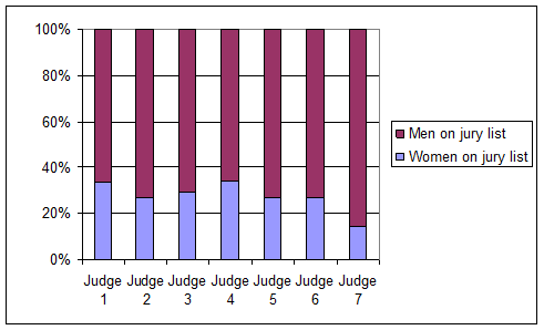
described in detail following the image
Segmented bar graph of each judge’s jury list split into women and men; Judge 7 shows a noticeably smaller proportion of women
There is some variability among the judges, but Judge 7 in particular has a much lower percentage of women on the jury list.
2. State Hypotheses.
Let \(\pi_i\) represent the (long-run) probability of judge \(i\) selecting a female for the jury list. State a null and an alternative hypothesis for testing whether these data provide reason to doubt that the probability of women on jury lists is the same for all seven judges.
Note: Your null hypothesis states only that the probabilities are equal; you are not specifying a particular value for this common probability. The alternative hypothesis can state only that at least one probability differs from the rest.
Solution.
\(H_0\!: \pi_1 = \pi_2 = \pi_3 = \pi_4 = \pi_5 = \pi_6 = \pi_7\)
\(H_a\!:\) at least one judge has a different long-run probability of selecting a female juror.

Choose a Statistic.

3. Propose a Statistic.
Suggest a statistic (formula based on your observed sample data) for assessing the strength of evidence against the null hypothesis.
Hint: Write your statistic as a formula or rule for obtaining one number that takes into account information in the sample relevant to comparing all seven groups.
Solution.
Answers will vary. Any reasonable statistic that summarizes how different the seven sample proportions are from one another could be proposed.
4. Pairwise Differences.
One possibility is to compare all the sample proportions to each other. We can do this by looking at all the pairwise differences, e.g., \(\hat{p}_{judge1} - \hat{p}_{judge2}\text{;}\) \(\hat{p}_{judge1} - \hat{p}_{judge4}\text{;}\) \(\hat{p}_{judge2} - \hat{p}_{judge4}\text{;}\) .... How many such pairs are there? Could we simply sum these differences?
Solution.
There are \({7 \choose 2} = 21\) pairs.
We would not want to simply sum the pairwise differences because positive and negative differences could cancel each other out.
Definition: Mean Group Difference.
One possible statistic for measuring how much the sample proportions differ from each other is the Mean Group Difference, which finds the absolute value of each pairwise difference \(|\hat{p}_i - \hat{p}_j|\text{,}\) sums these values, and divides by the number of differences.
5. Interpret Statistic Values.
What types of values do you expect this statistic to have when the null hypothesis is true? What about if the null hypothesis is false?
Solution.
Large values of a statistic that measures group differences would indicate evidence against the null hypothesis. Small values would be more consistent with the null hypothesis being true.
Although we could consider using the Mean Group Difference statistic here, a more common statistic is the chi-squared statistic. Rather than looking at all differences among the groups, it focuses on how each cell count differs from its expected value under the null hypothesis and then sums this up across all cells. This statistic generally has more power than the Mean Group Difference statistic and a nice predictable theoretical distribution.
6. Estimate Common Probability.
Assuming the null hypothesis is true, and each judge has the same probability of a female juror in his pool, suggest an estimate for this common (across all judges) probability that a juror is female.
Solution.
A reasonable estimate is the overall proportion of women in the combined data:
\(\hat{\pi} = 776/2975 \approx 0.261\text{.}\)
7. Expected Counts for Judge 1.
How many jurors were on Judge 1’s list? If you suppose the long-run proportion of women in his juries was 0.261, how many of these jurors would you expect to be female? How many would you expect to be male?
Recall: An expected value does not need to be an integer.
Number of jurors on Judge 1’s list:
Expected number of women:
Expected number of men:
Solution.
Expected number of women: \(0.261(354) = 92.39\)
Expected number of men: \(354 - 92.39 = 261.61\)
8. Expected Counts for Judge 2.
How many of the jurors on Judge 2’s list would you expect to be female if his long-run proportion was also 0.261? How many would you expect to be male?
Expected number of women:
Expected number of men:
Solution.
Expected number of women: \(0.261(730) = 190.53\)
Expected number of men: \(730 - 190.53 = 539.47\)
9. Complete Expected Counts Table.
Enter your expected counts below the observed counts in the following table.
Jury lists Judge 1 Judge 2 Judge 3 Judge 4 Judge 5 Judge 6 Judge 7
Women (Observed) 119 197 118 77 30 149 86
Women (Expected) 105.71 58.99 28.97 144.07 155.82
Men (Observed) 235 533 287 149 81 403 511
Men (Expected) 299.30 167.01 82.03 407.93 441.18
Solution.
The missing expected counts are:
Judge 1: women 92.39, men 261.61
Judge 2: women 190.53, men 539.47
The remaining expected counts are those already shown in the table.
10. Observed vs. Expected.
Are the observed counts equal to the expected counts in each cell of the table? Is it possible that the long-run probability of a female jury panel member is the same for each judge, and the differences between the observed counts and the expected counts found in the table are due to random chance alone?
Solution.
The observed counts and expected counts are not equal. However, that discrepancy could still be due to random chance alone, so we need to assess how unusual the overall discrepancy is under the null hypothesis.
Chi-squared Test Statistic.
The chi-squared test statistic is used to compare the observed and expected counts in a two-way table:
\begin{equation*} \chi^2 = \sum_{i=1}^{r} \sum_{j=1}^{c} \frac{(observed_{ij} - expected_{ij})^2}{expected_{ij}} \end{equation*}
where \(r\) = number of rows and \(c\) = number of columns. This standardized statistic looks at the discrepancy between the observed and expected counts for each cell, squares the difference to ensure a positive contribution, standardizes by dividing by the expected count, and then sums across all cells.
11. Compute Chi-squared Statistic.
Calculate this standardized statistic for the above two-way table.
\(\chi^2 =\) + + \(\frac{(118 - 105.71)^2}{105.71}\)
\(\qquad + \frac{(77 - 58.99)^2}{58.99} + \frac{(30 - 28.97)^2}{28.97} + \frac{(149 - 144.07)^2}{144.07} + \frac{(86 - 155.82)^2}{155.82}\)
\(\qquad +\) + \(+ \frac{(287 - 299.30)^2}{299.30}\)
\(\qquad + \frac{(149 - 167.01)^2}{167.01} + \frac{(81 - 82.03)^2}{82.03} + \frac{(403 - 407.93)^2}{407.93} + \frac{(511 - 441.18)^2}{441.18}\)
\(\chi^2 =\) + + \(1.43 + 5.50 + 0.04 + 0.17\)
\(\qquad + 31.29 +\) + \(+ 0.50 + 1.94\)
\(\qquad + 0.01 + 0.06 + 11.06\)
Hint.
Fill in the missing terms for the first two judges and then sum all of the values together.
Solution.
The four missing components are approximately:
\((119 - 92.39)^2/92.39 = 7.66\text{,}\) \((197 - 190.53)^2/190.53 = 0.22\text{,}\) \((235 - 261.61)^2/261.61 = 2.71\text{,}\) and \((533 - 539.47)^2/539.47 = 0.078\text{.}\)
Adding all components gives a chi-squared sum of approximately \(62.68\) (small differences can occur from rounding).
12. Direction of Evidence.
What types of chi-squared statistic values (large, small, positive, negative) constitute evidence against the null hypothesis of equal long-run probabilities? Explain.
Solution.
The chi-squared statistic is always nonnegative. Large values provide evidence against the null hypothesis; smaller values are more consistent with the null hypothesis being true.

Null Distribution.

In order to approximate the p-value of this test, we need to examine how the standardized statistic varies under the null hypothesis of equal probabilities. We will once again explore this null distribution first by simulating a large number of random samples where the probability of a juror being female is the same for each judge (under the null hypothesis).
13. Simulation Plan.
Outline the steps you would use to generate random data for each judge under the null hypothesis that the probability of a juror being female is the same for each judge.
Solution.
Generate random jury-list outcomes for each judge using the same probability of selecting a female juror, while keeping each judge’s sample size fixed. For each simulated data set, compute the chi-squared statistic. Repeat many times to build a null distribution of chi-squared values and compare the observed value to that distribution.
14. Describe Null Distribution.
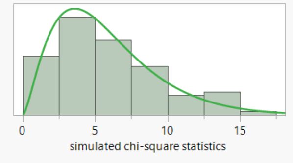
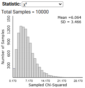
Describe the shape, center, and variability of the simulated null distribution.
Solution.
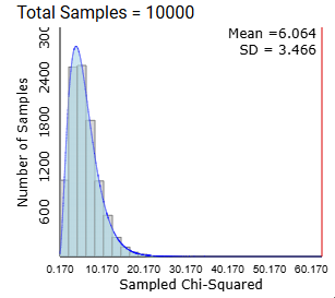
The simulated null distribution is skewed to the right. Its center should be around 6.
15. Empirical p-value and Conclusion.
Based on your simulation, determine the proportion of simulated standardized statistic values that are as large or larger than the standardized statistic value you computed in Question 11. Does this empirical p-value provide convincing evidence that the difference between observed and expected counts that you observed is larger than we would expect by chance? What do you conclude about whether the seven judges all had the same long-run probability of a juror being female? Explain.
Solution.
None of the simulated chi-squared values should be anywhere near \(62.68\text{,}\) so the empirical p-value is approximately 0.
This provides very strong evidence that the observed discrepancy is too large to attribute to random chance alone, so we conclude that the seven judges did not all have the same long-run probability of selecting a female juror.

Mathematical Model.

Rather than rely on simulation to produce (approximate) p-values for this test, we can use a probability model to approximate the sampling distribution of the chi-squared test statistic. We just need to find the right one.
16. Normal Model Check.
Does the normal probability distribution appear to adequately predict the behavior of the simulated null distribution of the chi-square statistic?
Solution.
No. The null distribution is skewed to the right, not approximately symmetric like a normal distribution.
17. Chi-squared Model Check.
Does this model appear to adequately predict the behavior of the simulated null distribution of this standardized statistic?
Solution.
Yes. The chi-squared distribution appears to be a reasonable model for this null distribution.
The chi-squared distribution is skewed right and provides a reasonable model for this statistic for large sample sizes. We typically use this model when all expected counts are at least 1 and at least 80% of expected counts are at least 5.
When comparing several population proportions, the chi-squared degrees of freedom are equal to the number of explanatory variable categories minus 1, \(c-1\text{,}\) this makes sense because once we specify the number of observations in \(c - 1\) categories, the last category is forced to assume the value that allows the observed counts to sum to the sample size.
For large sample sizes, we will use the chi-squared distribution to approximate the p-value.
Technology Detour.
18. Chi-squared Probabilities.
Use technology to calculate probabilities from a chi-squared distribution.
Hint 1. Applet Instructions
Use the Chi-squared Probability Calculator and specify degrees of freedom, observed value, and direction.
Hint 2. R Instructions
Use is.chisqprob(xval, df), where xval is the observed statistic and df is degrees of freedom.
Hint 3. JMP Instructions
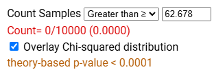
Use the Distribution Calculator and select the Chi Square distribution. Enter 6 as the degrees of freedom (DF) and press Enter. Leave the type of calculation to Input quantiles…. You want X > Qa and specify 62.68 for Qa.
Solution.
Example output:
First example output for chi-squared probabilities technology detour
Second example output for chi-squared probabilities technology detour
19. Compare p-values.
How does this p-value compare to the empirical p-value you determined in Question 15?
Solution.
Because the observed chi-squared statistic is so large, the model-based p-value is also approximately 0, so it agrees closely with the empirical p-value from the simulation.

Discussion.

If the null hypothesis is rejected, the conclusion we draw is that at least one of the population proportions differs from the rest, but we don’t have much information about which one. It could be that one explanatory variable group is behaving much differently than the rest or they could all be different. One way to gain more information about the nature of the differences between the \(\pi_i\) values is to compare the components of the chi-squared statistic sum.
20. Largest Chi-squared Components.
Return to the sum you calculated in Question 11. Which cell comparison(s) provide the largest (standardized) discrepancy between the observed counts and the expected counts?
Solution.
The largest contributions come from Judge 7’s cells.
21. Direction of Largest Discrepancies.
For the cells identified in Question 20, which is larger, the observed counts or the expected counts? Explain the implications of this comparison.
Solution.
For Judge 7, the observed number of women is less than expected and the observed number of men is greater than expected. This suggests that Judge 7 selected fewer women than would be expected under the equal-probability model.
22. Identify Judge in Spock Case.
Which judge do you believe tried Dr. Spock’s case? Explain.
Solution.
Judge 7. This judge stands out as having fewer women than expected, which matches the description of Judge Ford in Dr. Spock’s case.

Study Conclusions.

In this study, we wanted to think of the jury panel selection processes as independent binomial processes with potentially the same probability of success. We considered each of the venires we had as independent random samples from these different processes, and we wanted to compare the 7 sample proportions all at once. One judge clearly stood out compared to the others in these sample data. If we consider these results to be representative of the overall jury selection process, the very small p-value indicates that if in fact the judges’ selections of jurors were independent random processes with the same probability of selecting a woman, then it would be almost impossible to observe sample proportions differing by this much (as measured by the Mean Group Difference or the Chi-squared statistic) by chance alone. Thus, the sample data provide strong evidence that the long-run probability of a juror being female is not the same among all seven judges. The largest contributions to the \(\chi^2\) test statistic, by far, come from judge 7, who has many more men than would be expected and many fewer women than would be expected on his jury lists. This was indeed Judge Ford, the judge assigned to Dr. Spock’s case. In fact, there are two issues with this judge: The sampling from the city directory led to a far smaller percentage of women (29%) than the city population (53%) across all the judges, and then the proportion of women selected by Judge Ford dipped even lower to around 15% women. (By the way, the Court of Appeals reversed Spock’s conviction on other grounds without considering the jury selection issue.) Although this p-value is hypothetical in nature (there was not a true random mechanism used in generating these outcomes), and we cannot draw a cause-and-effect conclusion because of the observational nature of the data, the p-value does provides a measure of how very surprising these results would be to occur by chance alone.

Technical Conditions.

The chi-squared distribution approximates the sampling distribution of the chi-squared statistic when data arise from independent binomial random variables. This approximation is considered valid as long as at least 80% of the expected cell counts are at least 5 and all of the individual expected cell counts are at least one. Notice we are discussing the expected cell counts here, not the observed cell counts. The data also need to have been collected from independent random samples or from a randomized comparative experiment. This is often called a chi-squared test of homogeneity.
The advantage of a Chi-squared Test is that it provides an overall p-value for all the comparisons at once which controls the overall probability of a Type I error. If the p-value is not significant, we usually do not check all of the individual comparisons. If the p-value is significant, then we can do more formal follow-up analyses to see where the difference(s) are arising. If we run many tests on the same data set, we are always concerned about an inflated overall Type I error rate.

Technology Detour.

23. Simulating Sampling Distribution for Chi-Square Statistic.
Create a distribution of chi-square statistics and use probability plots to compare the simulated distribution to a theoretical model.
Hint 1. Applet Instructions
  • Load the Spock data into the applet and run the simulation.
  • Use the applet output to inspect the simulated chi-squared distribution.
Hint 2. R Instructions
Run Spock.R to generate chi-squared values.
  • To create a normal probability plot: qqnorm(chisqvalues)
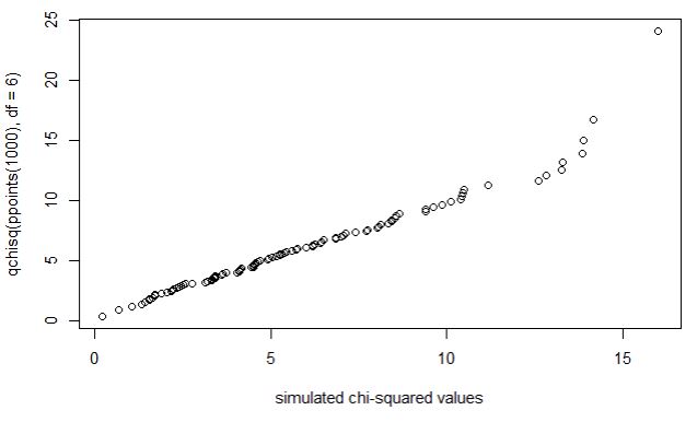
  • To create a QQ plot with values from a chi-squared distribution: qqplot(chisqsum, qchisq(ppoints(1000), df = 6))
Hint 3. JMP Instructions
Open Spock.jmp and run the simulation script.
  • To create a normal probability plot: choose Analyze > Distribution, select the chisqstat column, and then use the hot spot to select Normal Quantile Plot.
  • The chi-squared distribution is equivalent to a Gamma distribution with shape \(6/2 = 3\) and scale \(2\text{.}\) Use the hot spot to select Continuous Fit > Gamma.
Solution.
Applet.
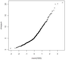
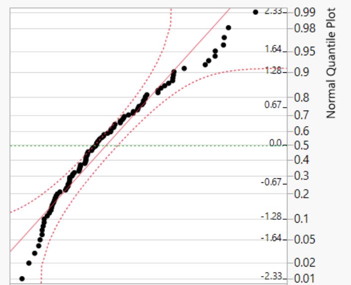
The normal quantile plot shows noticeable curvature rather than a straight-line pattern, so the simulated chi-squared values do not appear to follow a normal distribution well.
R.
The R output leads to the same conclusion: the normal probability plot bends upward in the right tail, which indicates right skew and suggests that a normal model is not appropriate for this null distribution.
Applet solution screenshot for chi-squared simulation
R solution screenshot for chi-squared simulation
JMP.
In JMP, the normal quantile plot again shows clear departure from linearity, reinforcing that the null distribution is not approximately normal.
JMP solution screenshot showing gamma fit workflow
Fitting the corresponding gamma distribution produces a much better match, which is consistent with using a chi-squared model for this statistic.
JMP solution screenshot showing normal quantile plot workflow

Subsection 24.1.2 Practice Problem 5.1

One question that you may be asking is why not just use the two-sample \(z\)-procedures to compare pairs of proportions? We could do this for two groups at a time, e.g., comparing Judge 1 to Judge 2 and then Judge 3 to Judge 5 and so on.

Checkpoint 24.1.24. Number of Comparisons.

How many such two-group comparisons are there among these 7 judges?

Checkpoint 24.1.25. Type I Error for One Comparison.

If the level of significance is set to 0.05, what is the probability of a Type I error for any one of these comparisons?

Checkpoint 24.1.26. At Least One Type I Error.

What about the probability of at least one Type I error among these 21 comparisons: will that be larger or smaller than 0.05? Explain.
You have attempted of activities on this page.