Skip to main content
Contents Index
Search Book
Search Results:
No results.
Calculator
Read aloud Readability settings Prev Up Next Scratch ActiveCode Profile title here \(
\newcommand{\lt}{<}
\newcommand{\gt}{>}
\newcommand{\amp}{&}
\definecolor{fillinmathshade}{gray}{0.9}
\newcommand{\fillinmath}[1]{\mathchoice{\colorbox{fillinmathshade}{$\displaystyle \phantom{\,#1\,}$}}{\colorbox{fillinmathshade}{$\textstyle \phantom{\,#1\,}$}}{\colorbox{fillinmathshade}{$\scriptstyle \phantom{\,#1\,}$}}{\colorbox{fillinmathshade}{$\scriptscriptstyle\phantom{\,#1\,}$}}}
\)
Section 16.4 Summary of Inference for Odds Ratio
RV \ EV
\(Group 1\) \(Group 2\)
\(Success\) \(A\) \(B\)
\(Failure\) \(C\) \(D\)
\(Total\) \(A + C\) \(B + D\)
Odds Ratio Procedures.
Statistic: Odds ratio (typically set up to be larger than one)
\begin{equation*}
\frac{A \times D}{B \times C}
\end{equation*}
\begin{equation*}
\frac{\text{odds}_1}{\text{odds}_2} = \frac{\hat{p}_1/(1-\hat{p}_1)}{\hat{p}_2/(1-\hat{p}_2)} = \frac{\hat{p}_1(1-\hat{p}_2)}{(1-\hat{p}_1)\hat{p}_2}
\end{equation*}
\(H_0\!: \tau = 1\) or
\(\ln(\tau) = 0\)
\(H_a\!: \tau < 1\text{,}\) \(\tau > 1\text{,}\) or
\(\tau \neq 1\) (or equivalently using
\(\ln(\tau)\) )
p-value: Fisher’s Exact Test or normal approximation on
\(\ln(\text{odds ratio})\)
Confidence interval for \(\tau\text{:}\) Exponentiate endpoints of
\begin{equation*}
\ln\left(\frac{A \times D}{B \times C}\right) \pm z^*\sqrt{\frac{1}{A}+\frac{1}{B}+\frac{1}{C}+\frac{1}{D}}
\end{equation*}
In Two-way Tables applet: Choose
Odds Ratio as statistic and check box for
95% CI
In R: fisher.test(matrix(c(a, c, b, d), nrow=2), alt = ) OR You can install the
fmsb package and use the
oddsratio command.
fmsb::oddsratio(A, B, C, D, conf.level, p.calc.by.independence = TRUE)
In JMP: From the Contingency Analysis hot spot, choose
Odds Ratio
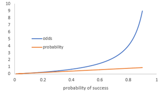
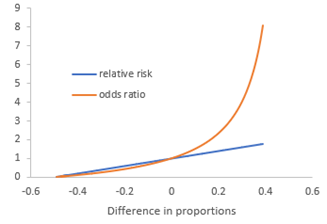
The graphs below show how (a) the probability of success and odds of success are related and (b) how relative risk and odds ratios are similar when the difference in proportions is small. Also note that when the difference in proportions is zero, the relative risk and the odds ratio are both one.
The table below demonstrates the invariance property of the odds ratio for
Investigation 3.9 . Notice that the odds ratio remains constant at 9.385 regardless of how we set up the comparison, while the relative risk changes depending on the setup.
Of lung cancer comparing smokers to non-smokers
\(\frac{583/576}{22/204} = 9.385\) \(\frac{583/1159}{22/226} = 5.17\)
Of not having lung cancer comparing non-smokers to smokers
\(\frac{204/22}{576/583} = 9.385\) \(\frac{204/226}{576/1159} = 1.816\)
Of not having lung cancer comparing smokers to non-smokers
\(\frac{576/583}{204/22} = 0.1065\) \(\frac{576/1159}{204/226} = 0.551\)
Of lung cancer comparing non-smokers to smokers
\(\frac{22/204}{583/576} = 0.1065\) \(\frac{22/226}{583/1159} = 0.194\)
Of being a smoker comparing lung cancer patients to controls
\(\frac{583/22}{576/204} = 9.385\) \(\frac{583/605}{576/780} = 1.305\)
See the
Technology Detour for instructions on simulating random assignment for two-way tables.
You have attempted
of
activities on this page.