Section 27.1 Investigation 5.10: Running Out of Time

Exercises 27.1.1 The Study

Many communities offer racing events for amateur runners, such as 5K (approximately 3.1 miles) races. At the end of the event, awards are often given out to runners with the fastest times, often to the top three finishers in different age groups. But does running time really change with age for amateur runners? To investigate this, one of the authors downloaded the race results for a local 5K race in May 2013 (Talley5K2013.txt). Data for 248 runners included age (in years) and finish time (in minutes).

1. Identify Variables.

Identify the explanatory and response variables for this research question.
Solution.
The explanatory variable of interest here is age and the response variable is finishing time.
2. Predict Direction, Form, Significance.

Do you expect the relationship between finish time and age to be positive or negative? Do you expect it to be linear (which implies what)? Do you think the association between these variables will be statistically significant?
Solution.
We might expect older people to tend to be slower (larger finish times) so a positive association. Conjectures about form and strength will vary.
  • Use technology to produce a scatterplot of finish time vs. age. [You can copy the data into Excel, using Data > Text to Columns and delimiting by spaces, and then copy the last two columns (age, time) into the Analyzing Two Quantitative Variables applet, using age as the explanatory variable.]

3. Produce Scatterplot.

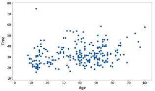
Do you want to change any of your answers to Question 2 in light of this graph? Also discuss any other unusual features of the data.
Solution.
Example output:
described in detail following the image
Scatterplot of finish time (minutes) versus age (years) for 248 runners, showing a weak positive association and one extreme outlier: a young runner with a time near 80 minutes.
We do notice a weak, positive, linear association between time and age. There is also an extreme outlier β€” a rather young runner who took almost 80 minutes. The outlier could be due to an injury during the race?
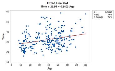
  • Remove the outlier from the data window (the name was a duplicate and the time was later dropped from the official published results, row #248), press Use Data again, and determine the least-squares regression equation for predicting finish time from age.

4. Remove Outlier; Regression Line.

Interpret the slope coefficient in context.
Solution.
Example output:
described in detail following the image
Fitted line plot of Time = 26.96 + 0.1403 Age with the outlier removed; S = 8.26529, R-sq = 7.6 percent, R-sq (adj) = 7.2 percent.
With each one-year increase in age, we predict about 0.1403 minutes to be added to the finish time, on average.

5. Could Association Be Chance?

Suppose we consider the remaining 247 runners to be a random sample from some larger population. Is it possible that there is no association between age and finishing time in this larger population, but we just happened to find such an association in this sample? How might we investigate how plausible this explanation is?
Solution.
It’s possible. We need to know how unusual a slope of .1403 (or more extreme) is for a random sample of 247 runners from a population with no association.

Terminology Detour.

To differentiate between the population regression line and the sample regression line, we will continue to use \(b_0\) and \(b_1\) to denote the sample statistics for the intercept and slope, respectively (or alternatively \(\hat{\beta}_0\) and \(\hat{\beta}_1\)). The corresponding population parameters will be denoted by \(\beta_0\) and \(\beta_1\text{.}\)

6. State Hypotheses.

If there were no relationship between finish time and age in the population, what would this imply about the value of the population slope? State null and alternative hypotheses to reflect the research question that 5K runner finishing times change with age. (Do you think they will increase or decrease?)
Solution.
This would imply a population slope of zero. \(H_0\text{:}\) no association between finish time (population slope = 0) and age vs. \(H_a\text{:}\) a positive association between finish time and age (population slope \(> 0\)).
We now want to assess the statistical significance of the association between variables in this sample. Following our usual logic, we will approach this question by assessing how unusual it would be to obtain a sample slope coefficient of \(b_1 = 0.140\) (or more extreme) with a random sample of 247 runners from a population with no association between the variables (i.e., with a population slope coefficient of \(\beta_1 = 0\)). We will do this by creating such a population and repeatedly taking random samples from it, calculating the sample slope each time.
First, let’s think about what we want this population to look like.

7. Sample Summary Statistics.

Determine the sample mean and standard deviation of the remaining individual variables in our sample (In the applet, you can check the Show descriptive box in the bottom left corner):
Finish time Mean = Standard deviation =
Age Mean = Standard deviation =
Also check the box to reveal the value of \(s\) from the regression model \(\sqrt{SSE/(n-2)}\text{:}\)
Regression SE =
Solution.
described in detail following the image
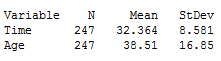
Descriptive statistics table: Time, n = 247, mean = 32.364, standard deviation = 8.581; Age, n = 247, mean = 38.51, standard deviation = 16.85.
Note: I removed the runner, not just the finishing time. \(s = 8.265\) min.
So one approach is to create a population that has similar characteristics as this sample, but with a population slope coefficient of zero.
Technical note: You also want to think about whether you want to model random sampling from a bivariate population, or random sampling of finishing times at each age. We will start with the first approach, but classical regression theory (Investigation 5.12) assumes the second.
In the Analyzing Two Quantitative Variables applet, check the Design Population box in the bottom left corner. Use the pull-down menu to select the Bivariate structure for the population (assumes normal distributions for both the explanatory and response variables). We will create a population of runners where there is no relationship between finish time and age. To match the above context:
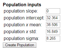
  • Use the mean of the time variable, 32.36, as the population intercept. Because we are forcing \(\beta_1 = 0\text{,}\) this says that the population regression line is constant at \(\bar{y} = 32.36\) minutes.
  • Use the \(x\) mean and \(x\) standard deviation to match the values you found in Question 7 for age after removing the outlier.
  • Use the standard error of the residuals as sigma, representing the variability about the population regression line (should be smaller than the SD(Y) you found in Question 7).
  • Press the Create Population button.
described in detail following the image
Population inputs panel of the Analyzing Two Quantitative Variables applet: population slope 0, population intercept 32.364, population x mean 38.506, population x std 16.849, population sigma 8.265, and a Create Population button.
Note: These values should appear in the applet when you check Create Population if you had pasted in the sample data first.
So the population of 20,000 runners we are creating here mostly matches the characteristics of the observed sample data. The key difference here is that we are assuming the population slope is equal to zero.
  • Check the Show Sampling Options box and set the sample size to be 247, choose the Slope as the statistic, and press the Draw Samples button. Make sure Show Regression Line is checked on the left

8. Draw One Sample.

Record the Most Recent Regression Line equation displayed in blue. Did you obtain the same sample regression line as from the observed race results (check the β€œShow Original Regression Line” box) or as in the hypothesized population (in light blue)?
Solution.
The sample regression line shouldn’t exactly match the population regression line (\(\beta_1 = 0\)).
  • Press the Draw Samples button again to get a new sample regression line (in blue, the previous turns grey).
These questions reveal once again the omnipresent phenomenon of sampling variability. Just as you have seen that the value of a sample mean varies from sample to sample, the value of a sample proportion varies from sample to sample, and the value of a chi-squared statistic varies from sample to sample, now you see that the value of a sample regression line also varies from sample to sample. Once again we can use simulation to explore the long-run pattern of this variation, approximating the sampling distribution of the sample slope coefficient.
  • Change the Number of Samples from 1 to 20. Press the Draw Samples button five times.

10. Twenty Samples.

Describe the pattern of variation that you see in the simulated regression lines.
Solution.
The lines form a criss-crossing pattern, like a bow-tie or cat whiskers.
  • Now change the number of samples to 1000 and press the Draw Samples button.

11. Null Distribution of Slopes.

Describe the shape, mean, and standard deviation of the null distribution of sample slopes.
Shape:
Mean:
Standard deviation:
Solution.
The shape should be symmetric with a mean around zero and a standard deviation of about 0.03.

12. Interpret the Mean.

Is the mean of this distribution of sample slopes roughly what you expected? Explain.
Solution.
We expect the average sample slope to be close to zero, the value of the population slope. This shows that the sample slope is an unbiased estimator of the population slope.
  • Now change the value of \(\sigma\) from 8.265 to 4.29 and press Create Population.

13. Decrease Sigma.

How does this change the scatterplot?
Solution.
The vertical distances from the points to the horizontal regression line will be smaller.

14. Predict Effect on Slope Distribution.

How do you think this will change the behavior of the distribution of sample slopes? (shape, center, variability)
Solution.
Conjectures will vary.
  • Press the Draw Samples button.

15. Check Conjecture (Sigma).

Was your conjecture in Question 14 correct? Be sure to comment on shape, center, and variability of the null distribution.
Solution.
There should be less sample-to-sample variability in the sample slopes (smaller standard deviation).
  • Change the value of \(\sigma\) back to 8.265 (and press Create Population) but now change the value of \(x\) std from 16.849 to 8.45. Press the Create Population button.

16. Decrease x Variability.

How does this change the population scatterplot? How do you think this will change the behavior of the distribution of sample slopes and the distribution of the sample intercepts?
Change to scatterplot:
Prediction:
Solution.
The horizontal distances from the points to the \(\bar{x}\) value will be smaller (less horizontal width to the population scatterplot). Predictions will vary.
  • Press the Draw Samples button.

17. Check Conjecture (x std).

Was your conjecture in Question 16 correct?
Solution.
There will actually be more sample-to-sample variability in the sample slopes (larger standard deviation).
  • Change the value of \(x\) std back to 16.849 (Press Create Population) and change the sample size from 247 to 125.

18. Decrease Sample Size.

Conjecture what will happen to the sampling distribution of the sample slopes.
Solution.
Might conjecture the sampling distribution to have less variability when the samples are based on larger sample sizes.
  • Press the Draw Samples button.

20. Summarize the Three Effects.

Summarize how each of these quantities affect the sampling distribution of the sample slope:
Solution.
With a larger value of \(\sigma\text{,}\) there is more variability in the distribution of sample slopes.
With a larger value of \(s_x\text{,}\) there will be less variability in the distribution of sample slopes.
With a larger sample size, there will be less variability in the distribution of sample slopes.
You should have made the following observations (when the technical conditions are met):
  • The distribution of sample slopes is approximately normal.
  • The mean of the distributions of sample slopes equals the population slope \(\beta_1\text{.}\)
  • The variability in the sample slopes increases if we increase \(\sigma\text{.}\)
  • The variability in the sample slopes increases if we decrease \(s_x\text{.}\)
  • The variability in the sample slopes decreases if we increase \(n\text{.}\)

21. Explain Intuition.

Explain why each of the last 3 observations make intuitive sense. [You may want to recall the pictures from the applet.]
Solution.
When there is less variation away from the regression line, there will be less variation in the sample regression lines, it is more difficult to get β€œextreme” sample regression lines.
When there is less variability in the explanatory variable, we are not given as much information about the relationship between the two variables and it will be easier to get more extreme sample results.
Larger samples, as we often see, lead to less sampling variability in our statistic.

22. Formula for SD of the Slope.

Are the last three observations consistent with the following formula for the standard deviation of the sample slope, \(SD(b_1)\text{?}\) Explain.
\begin{equation*} SD(b_1) = \sqrt{\frac{\sigma^2}{(n-1)s_x^2}} \end{equation*}
Solution.
Yes, \(n\) and \(s_x^2\) are in the denominator and \(s\) is in the numerator.
Back to the question at hand: Is it plausible that the observed sample slope (\(b_1 = 0.140\)) came from a population with no association between the variables and so a population slope \(\beta_1 = 0\text{?}\)

23. Assess Plausibility (slope = 0).

Return to (or recreate) the dotplot of the sample slopes for the first simulation. Where does 0.140 fall in this null distribution? Is it plausible that the population slope is really zero and we obtained a sample slope as big as 0.140 just by chance? How often did such a sample slope occur in your 1000 samples? In all the samples obtained by your class?
Solution.
Example results
described in detail following the image
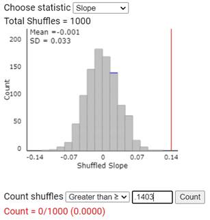
Histogram of 1000 simulated slopes with mean = -0.001 and SD = 0.033; counting slopes greater than or equal to .1403 gives Count = 0/1000 (0.0000), with the observed slope marked in the far right tail.
0.14 is in the tail of the simulated null distribution; it does not seem likely that if the population slope was zero we would observe a sample slope as extreme as 0.140 just by chance.
  • Change the population slope to .10 and press Create Population.
  • Draw 1000 samples and examine the new hypothesized population and the new sampling distribution of the sample slopes. (You may want to press Rescale.)

24. Assess Plausibility (slope = 0.10).

Where is the center? Roughly how often did you get a sample slope as big as 0.140 or bigger? Does it seem plausible that the students’ regression line came from a population with \(\beta_1 = 0.10\text{?}\)
Solution.
Example results
described in detail following the image
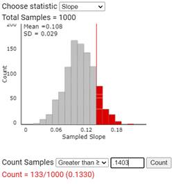
Histogram of 1000 sampled slopes with mean = 0.108 and SD = 0.029; counting samples greater than or equal to .1403 gives Count = 133/1000 (0.1330), with the region beyond the observed slope shaded.
The distribution of sample means will now center around 0.10. Now the value of 0.14 is not so extreme. Here we found such a slope or larger about 10% of the time. The value of 0.10 appears to be plausible for \(\beta_1\text{.}\)

Study Conclusions.

These sample data provide extremely strong evidence of a relationship between age and finishing time for the population of amateur runners similar to those in this sample. The above simulation shows that if there were no relationship in the population (\(\beta_1 = 0\)), then we would pretty much never see a sample slope as large as 0.140 just by chance (random sampling). We should be a bit cautious in generalizing these results to a larger sample as they were not a random sample. We might want to limit ourselves to 5K racers in similar types of towns.
The above simulation approach is a very intuitive way to assess the plausibility of a null hypothesis. However, it is not always practical to use this approach. In the next investigation, we will explore a more formal approach to assessing the plausibility of a null hypothesis in the regression setting.
As you have seen several times in this course, the sampling distribution of a statistic can often be well described by a mathematical model. This is also true in the regression setting. As when we focused on analyzing the individual population mean or comparing two population means, we need to first consider a way to estimate the (nuisance) standard deviation parameter.

25. Estimate the Standard Deviation.

If \(\sigma\) represents the common standard deviation of the response values about the regression line, suggest a way of estimating \(\sigma\) from the sample data.
Solution.
Suggestions will vary, but can use the \(s\) value calculated earlier.
If the conditions for the basic regression model (Investigation 5.12) are met, then if we standardize the sample slopes:
\begin{equation*} t_0 = \frac{b_1 - \beta_1}{SE(b_1)} \end{equation*}
where \(SE(b_1) = s\sqrt{\dfrac{1}{(n-1)s_x^2}}\) and \(s = \sqrt{\dfrac{\sum_{i=1}^{n}(residuals_i)^2}{n-2}}\text{,}\) these standardized values can be shown to be well approximated by a \(t\)-distribution with \(n - 2\) degrees of freedom. Note that we lose a second degree of freedom because we are estimating both the slope and the intercept from the sample data.

26. Compute the Standardized Statistic.

Using the standard deviation for the slopes you found in Question 23, calculate the standardized statistic.
Solution.
By hand: \(t = .14/.03 \approx 4.67\text{,}\) which will have a small p-value (\(df = 247 - 2 = 245\)).
Once we have the t-statistic or t-ratio, we can use the Student’s t-distribution to compute one- or two-sided p-values depending on the research question regarding the slope.

27. Compare with Technology.

Compare the t-ratio and p-value calculations based on the formula in Question 25 using technology.
Hint 1. R Instructions
Use summary(lm(time~age))
Hint 2. JMP Instructions
Analyze > Fit Y by X
Hint 3. Applet Instructions
Uncheck the Design Population box, and check the Regression Table box.
Solution.
The technology uses 0.0313 as the value of \(SE(b_1)\) rather than the estimate from the simulation, giving a t-value around 4.5.

Subsection 27.1.2 Practice Problem 5.10A

Checkpoint 27.1.1. Keep the Outlier.

Recreate this analysis (simulation as in Question 23 and t-test as in Question 26) without first removing the outlier. Do the results change much? If so, how? In the expected manner? Explain.

Subsection 27.1.3 Practice Problem 5.10B

The official published results for the 2013 race can be found online.

Checkpoint 27.1.2. Compare Datasets.

Load these data into your technology and then compare the two datasets.

Checkpoint 27.1.3. Identify a Second Difference.

Identify a second difference (apart from Scharlach_1 disappearing) between the unofficial and the official results.

Checkpoint 27.1.4. Compare Strength of Evidence.

How does the strength of evidence of a relationship between time and age differ for this dataset?
You have attempted of activities on this page.