With the proliferation of the Internet and 24-hour cable news outlets, it has become much easier for people to hear much more information, much more quickly. However, this has led to speculation that news organizations attempt to convey information before it has been properly verified in an effort to feed our impatience.
A “media believability survey” has been conducted since 1985 (under the direction of the Pew Research Center for the People & the Press since 1996), and research has focused on whether different news organizations (e.g., USA Today, NPR, MSNBC) have been losing credibility over time.
The survey is based on telephone interviews among a national sample of adults 18 years or older living in the continental United States. One of the questions asked is
Please rate how much you think you can BELIEVE each organization on a scale of 4 to 1. On this four point scale, “4” means you can believe all or most of what the organization says. “1” means you believe almost nothing of what they say. How would you rate the believability of (READ ITEM: ROTATE LIST) on this scale of 4 to 1?
Rotating the list helps prevent order effects. Without rotation, organizations listed earlier could be over-selected or rated differently simply because of position in the interview sequence.
Including cell phones reduces coverage bias. If only landlines are sampled, important groups (especially younger adults and cell-only households) are underrepresented.
Convert these percentages into observed counts among those who felt they could rate their daily newspaper. In other words, eliminate the “can’t rate” folks from consideration.
About 92.9% could rate the paper, so the count of raters is approximately \(1004(0.929) \approx 933\text{.}\) Converting the category percentages among raters gives counts of about 181 (rating 4), 371 (rating 3), 261 (rating 2), and 120 (rating 1).
Here the response variable is categorical with four ordered levels (an ordinal scale). In Investigation 5.1, the response variable was binary categorical (female/male).
A similar study was also done in 1998 (with 922 respondents able to rate their daily newspaper) and in 2012 (922 able to rate). A corresponding two-way table of counts across the three years is shown below.
The percentage declines from about \(265/922 \approx 28.7\%\) in 1998 to \(181/933 \approx 19.4\%\) in 2006, then is about \(183/922 \approx 19.8\%\) in 2012. So there is a large drop from 1998 to 2006 and little change afterward.
If the proportion who believe all or almost all of what they read was the same in all three populations, how many in the 2006 sample would you expect to believe all or almost all of what they read?
In general, we can calculate the expected count for each cell by considering the row and column totals corresponding to that cell. This ensures that the conditional distribution of the response variable is the same in each category of the explanatory variable.
State the null and alternative hypotheses for assessing whether the sample data provide strong evidence that the distribution of responses differs among the three years.
We will use the same Chi-squared statistic to compare the observed and expected counts, just now allowing for more than two categories for the response variable,
The applet reports the observed \(X^2\) value, df, and cell contributions. (You can expand this window by dragging out the lower right corner. Check the Show table box to see the observed counts.)
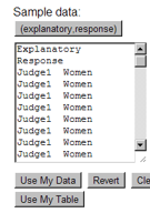
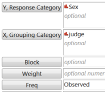
The data must be in “stacked format” (one column with the EV categories, one column with the RV categories). Each row can represent an observation or each row can represent a unique combination of variables and then you can add a column of counts (“tallied”).
Use technology to calculate the chi-squared statistic, verify the degrees of freedom, and calculate the p-value. Do you reject or fail to reject the null hypothesis?
A typical output gives \(\chi^2 \approx 45.22\) with \(df=(4-1)(3-1)=6\) and a very small p-value (\(p < 0.0001\)). We reject the null hypothesis and conclude that the believability distribution differs by year.
Use technology to carry out a chi-squared test to decide whether the difference in the population proportions giving a largely believable rating differed significantly between the two years. Report the standardized statistic, degrees of freedom, and p-value.
The chi-square test gives about \(\chi^2 \approx 19.9\) with \(df=1\) and \(p < 0.0001\text{,}\) indicating a statistically significant difference between years.
Now carry out a two-sided two-proportion \(z\)-test for this table. Report the standardized statistic and p-value. How do the p-values compare? What do you think is the relationship between the standardized statistics?
The two-proportion test gives about \(z \approx -4.46\) with a two-sided \(p < 0.0001\text{.}\) The p-values agree closely with the chi-square test, and the statistics satisfy \(z^2 \approx \chi^2\text{.}\)
The chi-squared procedure can be used to compare two or more proportions. When there are only two proportions, the procedure is equivalent to a two-sided \(z\)-test for proportions from Chapter 3. The chi-squared test statistic is equal to \(z^2\) and the chi-squared p-value is equal to the two-sided p-value for the two-sample \(z\)-test. If the alternative hypothesis is two-sided, you can use either procedure. If the alternative hypothesis is one-sided, then you should carry out the two-sample \(z\)-test to obtain the one-sided p-value. If there are more than two proportions, then you must use the chi-squared procedure, which will only assess whether or not at least one population proportion differs from the others.
For a \(2\times 2\) two-way table, another alternative is Fisher’s Exact Test as you learned in Chapter 3. It is always appropriate to carry out Fisher’s Exact Test (if you are willing to fix the row and column totals), though it may be a bit less convenient with huge sample sizes (which becomes less of an issue with each new computer chip).
However, of all three of these procedures, the two-sample \(z\)-procedure is the only one that also enables us to calculate a confidence interval to estimate the magnitude of the difference in the two population proportions.
Keep in mind that chi-squared tests look for evidence of any association. They don’t care which is the explanatory and which is the response and they don’t look for specific types of association, like time trend.
In February of 1993, NBC News admitted that it staged the explosion of a General Motors truck during a segment of the program “Dateline NBC” in November of 1992. The segment included crash footage that explosively showed how the gas tanks of certain old GM trucks could catch fire in a sideways collision. In a nationwide poll of adults (Times Mirror News Interest Index) conducted in August, 1989, 1507 respondents gave NBC news the following believability ratings.