Investigation 5.9: Money-Making Movies

Section 26.7 Investigation 5.9: Money-Making Movies

Exercises 26.7.1 The Study

Is there a tendency for movies that garner better audience reviews to also earn more money at the box office? The TopTenMovies.txt data file contains the world-wide movie gross, adjusted to be in 2015 dollars, for each movie, along with the IMDB rating (Source: https://www.crowdflower.com/data-for-everyone/).

1. Identify Study Variables.

Identify the observational units in this study. Also identify the explanatory and response variables, and classify them as categorical or quantitative.

Solution.

The observational units are the Top Ten movies, the explanatory variable is the IMDB ratings (quantitative) and the response variable is the box office revenue (quantitative).

2. Initial Scatterplot.

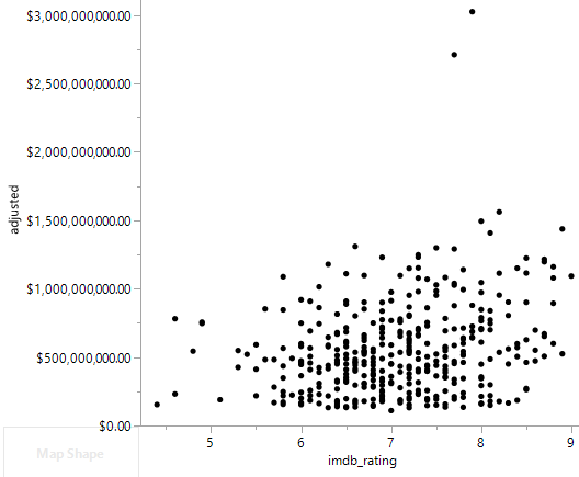
Produce a scatterplot to determine whether the IMDB rating appears to help predict the box office income (adjusted). Describe the relationship between the two variables as exhibited in the scatterplot.

Solution.

Scatterplot of adjusted box office revenue (in dollars) versus IMDB rating, showing a weak positive association with two very high revenue outliers.

If we treat box office revenue as the response variable there is a moderate positive linear relationship between box office revenue and the IMDB ratings.

3. Largest Residuals.

Identify the two or three points that you believe have the largest (in absolute value) residuals. Identify these movies by name.

Hint 1. Applet Instructions

In Two Quantitative Variables applet: You can mouse-click on an observation to reveal the row number. (You can also make movie the Color by variable and then mouse-click.)

Hint 2. R Instructions

You can use a command like movies[adjusted > 250, ]

Hint 3. JMP Instructions

Drag your mouse in the scatterplot to highlight the block of points. The rest will grey out. These observations will now be highlighted in the Data window. Use the Escape button in the Data window to unselect.

What does it mean for these movies to have such large residuals?

Solution.

The movies with the largest residuals are Titanic and Avatar. These movies had much higher box office revenues than we would have predicted based on the IMDB ratings.

4. Correlation Coefficient.

Determine, report, and interpret the value of the correlation coefficient.

Solution.

The correlation coefficient is $r = 0.269$ indicating a weakish, positive linear relationship.

5. Regression Equation.

Use technology to determine the least squares regression line for predicting the box office gross from the IMDB rating. Report the equation for this line. Also interpret the slope and intercept of this line in context.

Solution.

The regression equation is $\hat{income} = -232431603 + 109913810 \cdot imdb\_rating\text{.}$

The intercept is the predicted revenue (2015 dollars) if the IMDB rating is 0 (way below the minimum in our dataset).

The slope is the predicted increase in box office revenues (2015 dollars) associated with a 1 point increase in the IMDB rating.

The slope is rather small because the dollar amounts are so large. One way to improve the presentation of the results is to work with the response variable in millions of dollars.

6. Rescale Response.

Rescale the response variable to be in millions of dollars and repeat your analysis (scatterplot, correlation coefficient, regression line). How was the behavior of the scatterplot changed? The correlation coefficient? How have the slope and intercept changed? Could you have predicted these changes?

Solution.

New equation: $\hat{income} = -232.43 + 109.9 \cdot imdb\_rating\text{,}$ everything is now interpreted in terms of millions of dollars, but the association itself does not change form or strength.

7. Interpret r-squared and s.

Report the values of $r^2$ and $s$ and provide interpretations in this context.

Solution.

$r^2 = 7.25\%$ indicating that the regression on the IMDB rating explains about 7% of the variation in the box office revenues.

$s = 328.5$ indicating that this model predicts the box office revenue with a typical prediction error of about 328 million dollars.

Technology Detour.

8. Coded Scatterplot With Lines Instructions.

Create a coded scatterplot with a separate regression line for each MPAA rating category.

Hint 1. R Instructions

Create the coded scatterplot: plot(adjusted~imdb_rating, col=as.numeric(factor(MPAArating)))

Add the separate lines for each category, e.g.: abline(lm(adjusted[MPAArating=="G"]~imdb_rating[MPAArating=="G"]))

To cycle through the categories, create a column for the four categories and create a loop:

code=c("G", "PG", "PG-13", "R")
for (i in 1:4){
  abline(lm(adjusted[MPAArating==code[i]]~imdb_rating[MPAArating==code[i]]), col=i)
}

To add a legend: legend("topleft", legend=code, col=1:4, pch=1)

Hint 2. JMP Instructions

Choose Graph > Graph Builder.
Draw adjusted to the Y axis and imdb_rating to the X axis.
Select the 3rd icon to display the regression line.
Uncheck the box for Confidence of Fit.
Drag the “MPAArating” variable to the Overlay box.

Row of three JMP Graph Builder element icons; the third icon adds the regression line.

Hint 3. Applet Instructions

In Multiple Variables applet (or the Two Quantitative Variables applet for the color-coded graph alone)

Copy and paste the columns and press Use Data.
Drag adjusted to the Response box and imdb_rating to the Explanatory box. Drag MPAArating to the Subset by box.
Check the Show Equation box.
You can also check the box for separate graphs.

Solution.

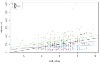
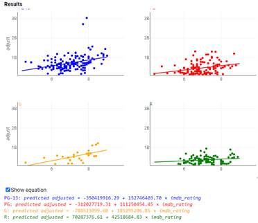
R and applet output

R coded scatterplot of adjusted revenue (millions) versus IMDB rating with separate regression lines and a legend for the G, PG, PG-13, and R rating categories.

Applet Results with four separate scatterplots by MPAA rating (PG-13, PG, G, R), each with its own regression line, and the Show equation output listing the four fitted equations.

9. Coded Scatterplot by MPAA Rating.

Describe what this coded scatterplot reveals about whether the relationship between box office income and IMDB ratings differs across the various MPAA rating categories. In particular, does any rating category tend to have higher box office values than you would expect for the score they received from IMDB reviewers? Is there a rating category tending toward lower box office revenues than expected? Explain.

Solution.

Most of the R movies are below the overall. The PG movies tend to be above the others with the same IMDB ratings. (Observations may vary a bit).

10. Coded Scatterplot by Genre.

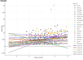
Repeat Question 8 using the primary movie genre (e.g., comedy) as the categorical variable (Genre_1). Summarize what you learn.

Solution.

Applet scatterplot of adjusted revenue versus IMDB rating with a separate regression line for each of the many Genre_1 categories, with a legend listing the genres.

Most of the Fantasy movies appear to earn more than predicted based on the IMDB ratings. (Observations may vary a bit). Would be fruitful to collapse the variable to a smaller number of categories.

11. Remove Two Highest-Revenue Movies.

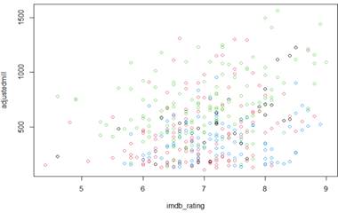
In analyzing these movies, the researchers also looked at the data set after removing the 2 movies that earned more than $2 billion. Subset the data (e.g., Investigation 2.1) and then examine the scatterplot, correlation coefficient, and least-squares regression line for predicting the movie income from the IMDB ratings for these data.

Solution.

Coded scatterplot of adjusted revenue (millions) versus IMDB rating after removing the two movies that earned more than 2 billion dollars.

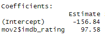
R coefficients output for the subset data: Intercept -156.84 and imdb_rating slope 97.58.

12. Effect of Removing Points.

Describe the effect of removing these 2 movies from the analysis.

Solution.

The slope is a little smaller and the correlation coefficient is a little larger ($R^2 = .075$), but overall, not much change. This is not a huge surprise given the size of the dataset and that the two observations did not have extreme values for the IMDB ratings.

Definition: Influential Observation.

An observation or set of observations is considered influential if removing the observation from the data set substantially changes the values of the correlation coefficient and/or the least squares regression equation. Typically, observations that have extreme explanatory variable outcomes (far below or far above $\bar{x}$) are potentially influential. To measure the influence of an observation, it is removed, and measures are calculated for how much the summary results change. It is not always the case that the points with the largest residuals are the most influential.

In this example you should have seen that removing those two movies does not noticeably impact the analysis results because they are not extreme in the $x$ direction.

Study Conclusions.

There does appear to be a weak relationship between the IMDB ratings and the amount of money the movie makes at the box office, with higher rated movies tending to make more money. If the IMDB rating increases by 1 point (out of 10), we predict the movie will make about 110 million more dollars. There are 2 clear outliers in terms of revenue (Avatar and Titanic) but they are not influential in the regression analysis. It is interesting that this model tends to underpredict revenues for PG-13 movies and overpredict revenues for R-rated movies, and that R-rating movies don’t seem as “impacted” by IMDB review scores. A next step in this analysis might be to collapse the number of Genre categories (e.g., combining Adventure, Animation, Fantasy categories, to see whether there is a tendency to underpredict their revenues).

Subsection 26.7.2 Practice Problem 5.9

Reconsider the idea of influential observations:

Checkpoint 26.7.2. Resistant Criterion.

Which do you think will be more resistant to outliers, the regression line that minimizes the sum of squared errors or the regression line that minimizes the sum of the absolute errors? Explain.

Checkpoint 26.7.3. Investigate with Applet.

Investigate your conjecture using the Analyzing Two Quantitative Variables applet. Write a short paragraph summarizing your analysis and your observations.

Subsection 26.7.3 Practice Problem 5.9B

Checkpoint 26.7.4. Rotten Tomatoes Predictor.

Repeat the analysis for the movie data using the Rotten Tomato scores (rt_score) to predict world-wide revenue. Summarize how the results compare.

You have attempted of activities on this page.

Prev Top Next