Section26.2Investigation 5.5: Restaurant Spending and Music
Exercises26.2.1The Study
A British study (North, Shilcock, & Hargreaves, 2003) examined whether the type of background music playing in a restaurant affected the amount of money that diners spent on their meals. The researchers asked a restaurant to alternate classical music, popular music, and silence on successive nights over 18 days.
State the null and alternative hypotheses corresponding to the researchers’ conjecture (in symbols and/or in words, be sure to define any symbols you use).
Based on these summary statistics, calculate the overall (weighted) mean amount spent, the between group variation, and the pooled variance. Check the consistency of your calculations with the summary statistics reported above.
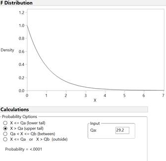
\(F = \frac{\text{between-group variability}}{\text{within-group variability}}\text{.}\) Using the values from earlier, this is approximately \(\frac{226}{7.73} \approx 29.2\) (minor differences may occur due to rounding).
The \(p\)-value is very small (approximately 0, depending on rounding and software display). The small p-value makes sense with the large (e.g., much larger than 4) \(F\)-statistic.
The variation between types of music appears larger than the variation in amount spent between diners. With \(F \approx 29.2\text{,}\) the between-group variation (types of music) is about 29 times larger than the within-group variation (between diners).
We would need to be able to verify the technical conditions (in fact, there is an issue here in that the treatments were assigned to the evenings and not the individual dinners).
In this study, a larger average amount was spent while classical music was playing. With such a large test statistic and such a small p-value (F = 29.2, p-value \(\approx\) 0), we have very strong evidence that the observed differences in the sample means could not have arisen by chance alone. However, we need to assess the technical conditions before we could know whether this inferential procedure is valid with these data. Although the equal standard deviation assumption seems reasonable (because 3.332/2.243 < 2), we do not have the sample data to examine the shapes of the sample distributions. Still, the sample sizes are large and the F procedure is fairly robust to departures from the normality condition. However, we should not consider these observations to be independent within each group, because the treatments were assigned to the evenings, not to the individual diners. In this sense, we only have a few replications per evening and ANOVA is not the appropriate analysis. Descriptively it appears that the average amount spent is larger when classical music is playing, but because of the confounding with evening, it’s possible that classical music was played on certain days of the week and that that led to more spending. This was a randomized experiment, so if it weren’t for the concern about independence, we would have been able to draw a cause-and-effect conclusion from the type of music played and the amount spent. We would want to be very cautious in generalizing these results to other restaurants and even other times of the year.
Another way to analyze the data for the trial of Dr. Spock is to look at the percentages of women on the different venires and determine whether the mean percentage of women is equal across the seven judges. Below are the percentages of women on the venires for a recent sample from each of the judges. These data are below and in SpockPers.txt.
Checkpoint26.2.1What New Information Does ANOVA Add?
Explain what information we learn from analyzing the data this way that we did not see when we carried out the Chi-squared test on the overall proportion of women for each judge. Why might this information be useful?
Carry out an ANOVA to test whether at least one judge has a different mean percentage. Did you state the null and alternative hypotheses in terms of population parameters or in terms of treatment effects?
Recall the Disability Discrimination study (Investigation 5.4). Suppose the researchers had been most interested in comparing the results for those in a wheelchair to those with leg amputation.
Carry out a two-sided two-sample pooled t-test (see the pooled \(t\)-test discussion in Investigation 4.2; use the technology option that assumes the variances are equal) to assess whether there is a statistically significant difference in the average ratings assigned to these two groups.
Carry out an analysis of variance to assess whether there is a statistically significant difference in the average ratings assigned to these two groups.
Checkpoint26.2.7Relate the \(t\) and \(F\) Results.
How are the p-values from Checkpoint 26.2.5 and Checkpoint 26.2.6 related? How do you think the t-test statistic and the F-test statistic are related? Explain.