Use technology (e.g., Multiple Variables applet) to determine the equation of the least squares line for predicting a cat’s takeoff velocity from its percentage of body fat (percentbodyfat). Record the equation of this line, using good statistical notation.
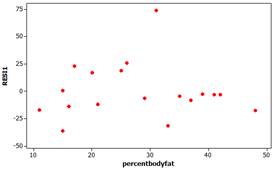
Examine a graph of the residuals vs. the percentage of body fat variable (or vs. the predicted values). Does the equal variance condition appear to be met? Does the linearity condition appear to be met?
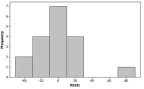
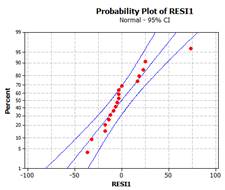
If we separate the one huge outlier, the remaining residuals are in a rectangular box from -25 to 25. The lack of any strong curvature indicates the linearity condition is reasonable and the lack of major “fanning” in the residuals indicates the equal variance condition is met.
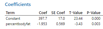
Consider testing whether the sample data provide strong evidence that percentage of body fat has a negative association with takeoff velocity in the population. State the hypotheses to be tested, and report (from the output) the value of the appropriate standardized statistic and p-value. (In the applet, check the Statistical model box.) Summarize your conclusion.
With a \(t\)-statistic of \(-3.343\) and a p-value of \(0.003 \lt .05\text{,}\) we would reject the null hypothesis at the 5% level of significance and conclude that we have convincing evidence of a negative association between percentage body and takeoff velocity in this population of cats.
Use a t-procedure and the values of \(b_1\) and \(SE(b_1)\) to produce (by hand) a 95% confidence interval for the population slope \(\beta_1\text{.}\)
If we use a \(t\) critical value for 95% confidence and \(18-2 = 16\) d.f, we would find \(-1.9534 \pm 2.1199(.5688)\) which gives \((-3.1592, -0.7476)\)
Interpret the confidence interval that you produced in Question 6. Be sure to interpret not only the interval itself but also what the slope coefficient means in this context.
Use the equation of the least squares line to predict the takeoff velocity for a cat with 25 percent body fat. Then do the same for a cat with 50 percent body fat.
Should have more faith in the prediction for 25% body fat as that value is in the main part of our data but we don’t have a lot of information for cats with body fat percentages around 50%.
Rather than only report one number as our prediction, we would like to specify a confidence interval that indicates how “accurate” or precise we believe our prediction to be. The following procedure is valid if the basic regression model conditions are met.
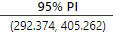
Report the 95% prediction interval for the takeoff velocity of a cat with 25% body fat. Also determine the midpoint of this interval; does its value look familiar? Also interpret what this interval reveals.
Use the predict command, passing in the variables for the linear model but also a “new data” data frame for the value(s) you want predictions for (but giving them the same name as your explanatory variable). For example:
JMP will add two columns to your table that use a Formula to compute the upper and lower endpoints of prediction intervals for all \(x\)-values of your data. Add new rows and enter new values for the explanatory variable to calculate prediction intervals for data other than those in the given dataset.
Midpoint is our prediction of 348.82. We are 95% confident that the takeoff velocity for a cat with 25% body fat will be between 292.37 cm/sec and 405.26 cm/sec.
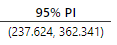
Repeat Question 10 to obtain a 95% prediction interval for the takeoff velocity of a cat with 50% body fat. Which interval is wider? Is this what you predicted in Question 9?
The midpoint is lower (now at 299.98) but the width is \(362.34-237.62 = 124.72\) (compared to \(405.26-292.37 = 112.89\)) is larger. This makes sense because we don’t expect predictions at 50% body fat to be as precise, but we expect lower take off velocity for these heavier cats.
As you saw in Investigation 2.6, the level of precision will also depend on whether we want to predict the mean response or an individual response outcome.
Statistical packages compute both “prediction intervals” and “confidence intervals.” A prediction interval gives us the interval of plausible values for an individual response at a particular value of the explanatory variable. A confidence interval gives us the set of plausible values for the mean response at a particular value of the explanatory variable.
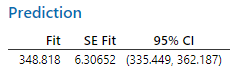
What does your technology report for the 95% confidence interval for the average takeoff velocity among all cats that have 25% body fat? Also determine the midpoint of this interval; does its value look familiar? Also interpret what this interval reveals.
The midpoint is the same (348.82). We are 95% confident that the average takeoff velocity for all cats with 25% body fat is between 335.45 and 362.19 cm/sec.
Technology tells us that we are 95% confident that a cat with 25% body fat would have a takeoff velocity between 292.4 and 405.3 cm/sec. But if we were to consider the population of all cats with 25% body fat, we are 95% confident that the mean takeoff velocity of these cats is between 335.5 and 362.2 cm/sec, a much narrower interval. These procedures are valid because the analysis of the residual plots did not reveal any strong departures from the basic regression model conditions.
Note: As with other t procedures, these procedures are fairly robust to departures from the normality condition if you have a larger sample size, except the prediction interval calculation.