In this investigation, you will learn about another probability distribution that allows you to calculate exact p-values when sampling from a population (rather than from a random process).
Concussions, particularly among high school and collegiate athletes, have been given increased attention in recent years. A 2017 national Youth Risk Behavior Survey found about 15.1% of U.S. high school students reported having at least one concussion in the previous year. Prevalence was higher among those who played on a sports team.
A student project group was interested in the probability of concussion among the male soccer and football players at their university. They sent a survey to the team rosters and found that 12 of the 33 respondents reported at least one concussion in the previous two years (2017–2019). The anonymous survey was emailed to all 110 players, and included a list of injuries asking "yes or no questions about various injuries, in order to distract the athletes of the true purpose of our survey." Based on these data, is there evidence that the proportion of all 110 male soccer and football players at this university who had at least one concussion in the last 2 years is larger than 0.15?
The response variable is Did the player have at least one concussion in the past 2 years? A "success" is having a concussion (or not having one - either is fine as long as you are consistent throughout the Investigation).
Non-sampling errors can occur even after we have a randomly selected sample. They are not associated with the sampling process, but rather with sources of bias that can arise after the sample has been selected.
Sources of non-sampling errors in surveys include biased, dishonest, or inaccurate responses by respondents due to leading word choice in survey questions, sensitive questions, faulty memory, the order in which questions appear, a leading tone, and the appearance of the interviewer.
Do you think it is reasonable to consider this sample as representative of all varsity team football and soccer players at this school? Explain why or why not.
It is unlikely to be representative of all football and soccer players at this university. The responses were voluntary and therefore this was not a random sample, and the response rate was low (0.3).
We can still ask: "If the population proportion was 0.15, would it be unlikely for a random sample from this population to produce such a large sample proportion?" This question should sound familiar, but now we need to consider that the sample did not come from a large population and this can impact our estimate of the amount of random sampling variation.
Suppose 17 of the 110 male football/soccer players at this school suffered a concussion. If we randomly select one of these athletes, what is the probability he had a concussion?
You should find your answers in Question 9 are not quite the same. This illustrates a violation of the independence assumption of our binomial model. However, if the population is large compared to the size of the sample, then the conditional probabilities are almost equal, and we can approximate with a binomial distribution. But when the population is not large, we need to take that lack of independence into account.
When sampling without replacement from a finite population that is not more than 20 times the size of the sample, the "trials" are no longer independent.
The consequence is that we should not use the binomial distribution to calculate \(P(X \geq 12)\text{.}\) Instead of a calculation like \(\binom{33}{12}(0.155)^{12}(1-0.155)^{21}\text{,}\) we would need a calculation like
When outcomes are equally likely, then the probability of an event equals the number of ways for the event to happen divided by the total number of possible outcomes.
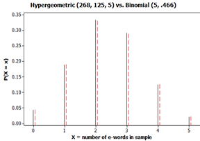
For example, there are 268 words in the Gettysburg Address, 125 contain the letter e (about 46.6%) and 143 do not. Using counting rules, there are \(\binom{268}{5} = 11,096,761,368\) different samples of 5 words that we could select from the Gettysburg Address. But if we want to select one e-word and four non-e-words, there are \(\binom{125}{1} \times \binom{143}{4} = 2,087,710,625\) such samples. Thus, if \(X\) = number of e-words in a sample of 5 words, we find \(P(\text{one e-word}) = P(X = 1) = 2,087,710,625 / 11,096,761,368 \approx 0.188\text{.}\)
The main distinction between a hypergeometric random variable and a binomial random variable is the trials are no longer independent. The probability of drawing a success for the first object is \(M/N\text{.}\) But if we do draw a success, then the probability of success for the second object is \((M - 1)/(N - 1)\text{.}\) If we replaced the item, then we would be back to a binomial process.
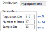
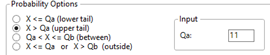
Continuing to suppose 17 of the 110 athletes had a concussion, use technology to find the probability that a random sample of 33 would have 12 or more successes.
If 15.5% of all football and soccer players at this university have had a concussion during the past two years, the chance we would find at least 12 of a random sample of 33 of these athletes reporting a concussion is 0.0002.
This sample was not randomly selected from the population of all U.S. collegiate football and soccer players, so this sample really tells us nothing about the likelihood of a concussion among the larger population.
The hypergeometric distribution is able to tell us that if we listed all possible samples of 33 players from this population, how many would be at least as extreme as the observed sample. In many sampling situations, our population size is large enough that the binomial distribution gives a very reasonable approximation to the exact p-value. For this reason, the binomial p-value is much more commonly used than the hypergeometric p-value.
These probability calculations work out to be very similar! This happens when the finite population we are sampling from is large compared to our sample size (e.g., \(N > 20 \times n\)). This means we can continue to use the binomial distribution to determine such probabilities and the expected number of successes \(5(0.466) \approx 2.33\) with \(SD(X) \approx 1.115\) successes. And when the sample size is large relative to the probability of success, we can approximate the binomial with the normal distribution.
Only about 0.02% of random samples of 33 players from a population of 110 players with 17 successes would have 12 or more successes in the sample by random chance (random sampling) alone. This survey would give us very strong evidence that the proportion of players with at least one concussion in this population was larger than 0.151, but there are many problems with this conclusion. This was not a random sample from the population of all athletes at this school (voluntary response, no follow-up) and is likely susceptible to sampling bias. Perhaps athletes who recently had a concussion would be more motivated to voluntarily complete the survey. Because of these issues with the sampling method, the p-value that we calculated is really not all that appropriate or meaningful. We should also consider that the 15% value cited by the YRBS came from one year of data vs. during the previous two years. Nevertheless, getting accurate reports on concussion rates is a challenging but critical task in helping to prevent possibly debilitating injuries, especially in high contact high school and college sports.
A 2004 student project asked 30 students from the 705 first-year students at their school whether they planned to vote for Bush or Kerry in the upcoming election. For half of the surveys, Kerry was listed first and for half of the surveys Bush was listed first. (Why?) They found 22 planned to vote for Kerry. Does this convince you that more than 2/3 of first-year students at this school planned to vote for Kerry?
Recall the GSS survey in Practice Problem 1.14. Identify potential non-sampling errors in such a study. What are some steps the GSS has taken/could take to avoid non-sampling errors?