Exercises 26.1.1 The Study
The U.S. Vocational Rehabilitation Act of 1973 prohibited discrimination against people with physical disabilities. The act defined a disabled person as any individual who had a physical or mental impairment that limits the person’s major life activities. In 1984, disabled individuals in the labor force had an unemployment rate of 7% compared to 4.5% in the non-impaired labor force.
Researchers conducted a study in the 1980s that examined whether physical disabilities affect people’s perceptions of employment qualifications (
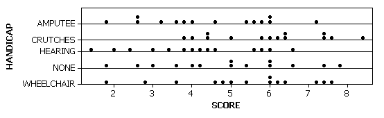
Cesare, Tannenbaum, & Dalessio, 1990). The researchers prepared videotaped job interviews, using the same actors and script each time. The only difference was that the job applicant appeared with different disabilities:
Seventy undergraduate students from a large southeastern university were randomly assigned to view one of the videotapes, and they were then asked to rate each candidate on ten questions (e.g., applicant is qualified, applicant likely to be productive) using a 1-9 scale (e.g., 1 = typical response of an applicant likely to be rejected, 9 = typical response of an applicant likely to be hired). The responses were averaged across the 10 questions as an overall rating of each applicant. The research question is whether subjects tend to evaluate qualifications differently depending on the applicant’s disability.
1. Identify Study Components.
Identify the observational units, explanatory variable, and response variable in this study. Identify each variable as quantitative or categorical. Is this an observational study or an experiment? Explain.
Solution.
The observational units are undergraduate students.
The explanatory variable is the type of disability and the response variable is the rating of candidate’s qualifications.
This is an experiment as the undergraduate students were randomly assigned to view one of the types of disabilities.
2. State Hypotheses.
State a null and an alternative hypothesis to reflect the researchers’ conjecture. Be sure to define any parameter symbols you use.
Solution.
Let
\(\mu_i\) = the true treatment effect for disability type
\(i\text{.}\)
\(H_0\!: \mu_{amp} = \mu_{crutch} = \mu_{hear} = \mu_{none} = \mu_{wheel}\)
\(H_a\!:\) at least one of the
\(\mu\)’s differs from the rest.
3. Type I and Type II Errors.
Explain what a Type I error and a Type II error represent in this context.
Solution.
Type I Error = thinking there is a difference in the effect of the disability types when there is not.
Type II Error = thinking there is a not a difference in the effect of the disability types when there is.
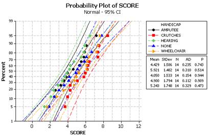
The mean applicant qualification scores for the five groups are amputee 4.429, crutches 5.921, hearing 4.050, none 4.900, and wheelchair 5.343.
4. What Else Is Needed?
What additional pieces of information do you need in order to decide whether these sample means are significantly different (more than you might expect by the random assignment process alone)?
Solution.
Sample sizes, degree of overlap of the two distributions.
5. Propose Statistic and Simulation.
-
Suggest a standardized statistic that you could use to measure how much these five sample means differ.
-
Outline a simulation you could perform to create a null distribution for your statistic.
-
What types of values of your statistic will you consider evidence against the null hypothesis (large, small, near 0)?
Solution.
Suggestions for statistic will vary but consider statistics involving deviations of the sample means from the overall mean or deviations of the sample means from each other. Then you would reassign the response outcomes to the disabilities (mimicking the random assignment process), calculate the statistic, repeat many times and see how often you get a statistic at least as extreme as what the researchers observed in this study. If you used a Mean Absolute Difference or Sum of Squared Deviations type of statistic, this would be closer to zero when the null hypothesis is true and large values would be evidence against the null hypothesis.
For example, we could put the 70 rating scores on index cards and then randomly assign 14 cards to 5 different groups and see what value of the chi-squared test statistic we get for each randomization.
One approach is to use a
Mean Group Difference, similar to what we discussed in Section 5.1, and to simulate the re-assigning of the given employment rating scores to the five types of disabilities.
-
-
Copy and paste the raw data (
DisabilityEmployment.txt) or type DisabilityEmployment.txt in the data window, being sure to clarify which is the explanatory variable, and press
Use Data.
-
Check the
Show Shuffle Options box.
-
Select the
Plot radio button and press
Shuffle Responses.
6. Interpretation.
What random process is the applet simulating?
Solution.
Random assignment of subjects to disabilities.
-
Change the
Number of Shuffles to a large number and press
Shuffle Responses.
7. Empirical p-value from Mean Group Diff.
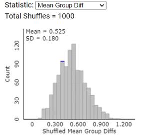
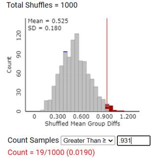
Examine the null distribution of the Mean Group Diff statistic and determine a simulation-based p-value.
Solution.
Example results:
The distribution will have a slight skew to the right, be centered around 0.5, with a standard deviation of around 0.2. Observed Mean Group Diff = 0.931.
A New Statistic.
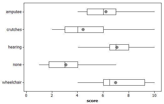
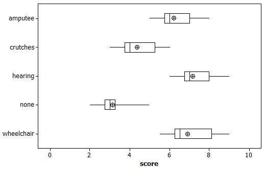
Consider the following sets of boxplots.
8. Compare Two Sets of Boxplots.
What is the same and what is different about the distributions displayed by these boxplots? In which group do you believe the evidence will be stronger that at least one population mean differs from the others? Explain. How will the Mean Group Difference statistics compare?
Solution.
The means (and sample sizes) are the same but the "within group" variability (spread of the individual distributions) differs. The observations in B are more consistent (smaller sample standard deviations). This should provide stronger evidence that the difference in group means is not just by random chance alone. The Mean Group Diff statistic is the same in both cases because it only examines the differences in means.
Discussion.
In the above boxplots, the sample mean scores are roughly the same for graphs A and B (6.2, 4.4, 7.1, 3.1, 7.0), but the variability within each group is much larger for the distributions in graph A. This larger amount of “within-sample” variation makes the differences in sample means seem not as extreme compared to graph B. Graph B displays less within-sample variability and so the differences in the sample means appear more extreme and provide more evidence that the crutches scores and the hearing scores did not come from the same population with the same population mean. So rather than reporting only the Mean Group Difference statistic, we will now explore another “standardized” statistic that is more meaningful on its own and, turns out, has more power. Our goal will be for this statistic to reflect not only the differences in the sample means, but to also reflect the “natural variation” in the data themselves.
9. Record Descriptive Statistics.
Record the missing descriptive statistics in the table below.
Solution.
SDs: 1.794, 1.586, 1.482, 1.533, 1.748.
10. Interpret SD for None Category.
Write a one sentence description of the sample standard deviation of the none category.
Solution.
This tells us that there was variability in the ratings giving to the "none" candidate by the 14 students who viewed that tape. Most of the ratings were within 1.794 of the mean rating. This was one of the more variable categories.
This time, rather than focusing on differences in groups, we will examine deviations in the group means.
11. Overall Mean.
What is the overall mean applicant qualification rating assigned by the 70 students?
Solution.
The overall mean is 4.929.
12. SD of Group Means.
If we were to treat the five sample means as five observations, calculate the standard deviation of these five values. What is the denominator of your calculation?
Solution.
\((4.9 - 4.929)^2 + (4.429 - 4.929)^2 + (5.921 - 4.929)^2 + (4.050 - 4.929)^2 + (5.343 - 4.929)^2\) divided by 4, and then taking the square root:
\(0.738\text{.}\)
The variance would be not taking the square root, approximately
\(0.545\text{.}\)
Recall: Squaring the standard deviation gives us the
variance of the values.
13. Equal Contribution of Means?
Is it reasonable to allow each of these sample means to have the same relative contribution to our overall measure of variability between group means? Explain.
Solution.
Yes, because the sample sizes are all equal.
Our measure of the variability between groups or “treatment effect” will be the weighted variance across the groups where the weights are the sample sizes.
\begin{equation*}
\frac{n_1(\bar{x}_1 - \bar{x})^2 + n_2(\bar{x}_2 - \bar{x})^2 + n_3(\bar{x}_3 - \bar{x})^2 + n_4(\bar{x}_4 - \bar{x})^2 + n_5(\bar{x}_5 - \bar{x})^2}{5 - 1}
\end{equation*}
14. Between-group Variability (Equal \(n\)’s).
In this case, the sample sizes were equal to 14 in each group, so you can simply multiply your answer to
Question 12 by 14 to measure the variability between groups.
Solution.
\(14(0.545)=7.63\text{.}\)
But now we want to compare this variation to decide if it’s large, more than we might expect to see by random chance alone, reflecting that not everyone gives the same rating scores, even to the same applicant.
15. Measure Natural Variation.
Suggest a way for measuring this “natural” variation for these data.
We could look at the variation in employment ratings (e.g., overall standard deviation), but some of that variation is due to the different types of disabilities. However, we can look at the variation in the ratings within each type of disability. If we believe these variances are the same, we can simply average across the categories, paying a bit more attention to any categories with more observations. (You considered something similar back in
Investigation 3.5)
16. Within-group Variability.
Calculate the average variance across the five groups.
Hint.
Square each group’s standard deviation to obtain its variance, and then take the average of those five values.
Solution.
average variance =
\((1.586^2 + 1.482^2 + 1.533^2 + 1.794^2 + 1.748^2)/5 = 13.3357/5 = 2.67\text{.}\)
When the sample sizes are not equal, the more general formula for this pooled variance, weighted by sample size, is:
\begin{equation*}
s_p^2 = \frac{(n_1-1)s_1^2 + (n_2-1)s_2^2 + (n_3-1)s_3^2 + (n_4-1)s_4^2 + (n_5-1)s_5^2}{(n_1 -1) + (n_2 -1) + (n_3 -1) + (n_4 -1) + (n_5 -1)}
\end{equation*}
This provides an overall estimate of the “within-group” variability, which simplifies to the average of the group variances when the sample sizes are equal. The denominator simplifies to
\(n – I\text{,}\) where
\(n\) is the total number of observations in the data set and
\(I\) is the number of groups being compared.
17. Equal Variability Assumption.
In calculating a pooled variance, you are implicitly assuming that the variability is the same across the groups. Explain how the sample statistics reveal that this is a reasonable belief for these data.
Solution.
The sample standard deviations reported in
Question 9 are fairly similar to each other.
Our standardized statistic will consider the ratio of the variability between groups to the variability within groups.
18. Compute Variability Ratio.
F = between-group variability / within-group variability
How many times larger is the between-group variability compared to the within-group variability?
Solution.
\(7.63/2.67 = 2.86\text{;}\) the between group variation is almost 3 times larger than the "natural" variation in these data.
19. Range of Ratio.
What is the smallest possible value that this ratio could ever assume? The largest?
Solution.
Smallest value is zero which would result if there was no between group variation. There is no upper bound on the value this ratio can assume.
20. Evidence Direction for Ratio.
What types of values (large, small, positive, negative) will this ratio have when the null hypothesis is false, that is, when the population means are not all equal?
Solution.
This ratio will be large when the null hypothesis is false and small when it is true (but always nonnegative). In fact, when
\(H_0\) is true, the ratio should be approximately one.
-
In the Comparing Groups (Quantitative) applet, use the pull-down
Statistic menu to select
F-statistic (named after R. A. Fisher).
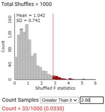
21. F-statistic Null Distribution.
Describe the behavior of the null distribution and compute the empirical p-value.
Solution.
The shape is skewed to the right with a mean around 1 and SD around 0.7.
22. Compare p-values Across Statistics.
Has the p-value changed much from when we used the Mean Group Difference statistic?
Solution.
This p-value is similar (but a bit larger) than we found with the Mean Group Difference statistic.
Probability Result.
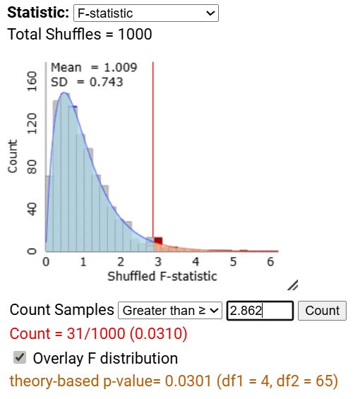
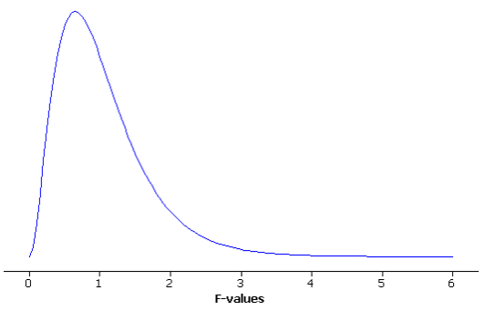
For large samples, this sampling distribution is well modeled by an
F distribution with parameters
number of groups − 1 and
overall sample size −
number of groups, the degrees of freedom of the numerator and denominator respectively.
23. Overlay F Distribution.
Check the Overlay
F distribution box. Does it appear to provide a reasonable approximation to the simulated null distribution? How are you deciding?
Solution.
We see that the
F distribution provides a good model of the simulated null distribution.
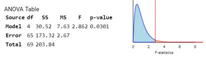
24. ANOVA with Technology.
Confirm your calculations using technology. Because we are comparing variances, this is called an
Analysis of Variance or
ANOVA procedure.
Technology Detour — ANOVA.
Hint 1. Applet Instructions
-
Paste data into Sample data box, being sure to clarify which is the explanatory variable.
-
-
Check the
Show ANOVA Table box.
Hint 2. R Instructions
If you have the data in a response vector and an explanatory vector, you can use
summary(aov(response~explanatory))
This will output the Mean Square values in the Mean Sq column, first for the treatment group (the disability row) and then for the error term (Residuals).
Hint 3. JMP Instructions
-
With the quantitative variable in one column and the explanatory variable in another column, choose
Analyze > Fit Y by X.
-
Specify the quantitative variable in the
Y, Column box and the explanatory variable in the
X, Factor box.
-
Open the
Oneway Analysis hot spot and select
Means/Anova.
Technical Conditions.
There are several technical conditions required for this randomization distribution to be well modeled by the
F distribution:
-
The distribution for each group comes from a normal population.
-
The population standard deviation is the same for all the groups.
-
The observations are independent.
When using this ANOVA
F-test to compare several population means, we will check each condition as follows:
-
The normal probability plot (or dotplot or histogram) for each sample’s responses is reasonably well-behaved.
-
The ratio of the largest standard deviation to the smallest standard deviation is at most 2.
-
The samples are independent random samples from each population.
For simplicity, we will apply the same checks for a randomized experiment as well (with the last condition being met if the treatments are randomly assigned). If the first two conditions are not met, then suitable transformations may be useful.
25. Check Conditions with Data.
Is there evidence of non-normality in these sample data? Calculate the ratio of the largest to smallest standard deviation; is this less than 2? (In the applet, check the box to Overlay
F distribution to help assess the fit.)
Solution.
There is no evidence of nonnormality and the ratio of the largest to smallest sample standard deviation (
\(1.794/1.482\)) is less than 2.
26. Conclusions Paragraph.
Write a paragraph summarizing your conclusions for this study. Be sure to address issues of causation and generalizability as well as statistical significance.
Solution.
There is moderate evidence that these average qualification ratings differ more than we would expect from the randomization process alone. There is at least one disability that has a different effect on the qualification ratings than the other disabilities. The ANOVA procedure appears valid since the observed treatment group distributions look reasonably normal and treatment group standard deviations are also similar.
Terminology Detour.
We will compare
\(I\) group means, where each group has
\(n_i\) observations. The overall sample size will be denoted by
\(n=\sum n_i\text{.}\)
\(H_0\text{:}\) There is no treatment effect or
\(H_0\!: \mu_1 = \cdots = \mu_I\)
\(H_a\text{:}\) There is a treatment effect or
\(H_a\!:\) at least one
\(\mu_i\) differs from the rest
The between-group variability will be measured by looking at the sum of the squared deviations of the group means to the overall mean, \(\bar{x}\text{.}\) Each group mean is weighted by the sample size of that group. We will refer to this quantity as the “sum of squares for groups,” SSgroups.
\begin{equation*}
SS_{groups} = \sum_{i=1}^I n_i(\bar{x}_i - \bar{x})^2\text{.}
\end{equation*}
We will then “average” these values by considering how many groups were involved. This quantity will be referred to as the “mean square for groups.”
Note, if we fix the overall mean, once we know
\(I - 1\) of the group means, the value of the
\(i^{th}\) mean is determined. So the degrees of freedom of this quantity is
\(I - 1\text{.}\)
The within-group variability will be measured by the pooled variance. In general, each term will be weighted by the sample size of that group. We will again divide by an indication of the overall sample size across the groups. We will refer to this quantity as the “mean squares for error,” MSE.
\begin{equation*}
MSE = \frac{\sum_{i=1}^I (n_i - 1)s_i^2}{n - I}
\end{equation*}
which has \(n - I\) degrees of freedom.
The test statistic is then the ratio of these “mean square” quantities:
When the null hypothesis is true, this test statistic should be close to 1. So larger values of
F provide evidence against the null hypothesis. The corresponding p-value comes from a probability distribution called the
F distribution with
\(I - 1\) and
\(n - I\) degrees of freedom.
We will use this
F distribution to approximate both the sampling distribution of this test statistic in repeated samples from the same population (
\(H_0\!: \mu_1 = … = \mu_I\)) and the randomization distribution for a randomized experiment (
\(H_0\!:\) no treatment effect) as long as the technical conditions (above) are met.
Because we are focusing on the variance of group means, this procedure is termed Analysis of Variance (ANOVA). With one explanatory variable, this is called
one-way ANOVA.
Study Conclusions.
The distributions of qualification scores in the five treatment groups look reasonably symmetric with similar standard deviations, so it is appropriate to apply the Analysis of Variance procedure. There is moderate evidence that the mean qualification ratings differ depending on the type of disability (p-value = 0.030). Descriptively, the candidates with crutches appear to have higher ratings on average, and the candidates with hearing impairments tend to have slightly lower ratings. (Other follow-up procedures could be used to determine which group means differ significantly from which others.) This was a randomized experiment, so we can attribute these differences in qualification scores to the disability shown. But we must be cautious about considering the students in this study to be representative of a larger population, particularly a population of employers who make actual hiring decisions.