Section27.4Investigation 5.8: Height and Foot Size
Exercises27.4.1The Study
Criminal investigators often need to predict unobserved characteristics of individuals from observed characteristics. For example, if a footprint is left at the scene of a crime, how accurately can we estimate that person’s height based on the length of the footprint? To investigate this possible relationship, data were collected on a sample of students in an introductory statistics class.
A residual is the difference between the predicted value and the observed value. If we let \(y_i\) represent the \(i\)th observed value and \(\hat{y}_i\) represent the predicted or “fitted” value, then
Show mathematically that the sum of residuals from the sample mean for any dataset equals zero. In other words, show that \(\sum_{i=1}^{n}(y_i - \bar{y}) = 0\text{.}\)
Suggest two ways to get around the problem revealed in Question 7 and Question 8. In other words, suggest something related to but different from summing residuals to use as a useful measure of overall prediction error.
Suppose that you want to use a single number (call it \(m\)) for predicting height. Use calculus to determine \(m\text{,}\) as a function of the data \(y_i\)’s, to minimize the sum of squared residuals from that prediction. Interpret your answer for \(m\text{.}\)
You are choosing \(m\) to minimize \(S = \sum_{i=1}^{n}(y_i - m)^2\text{.}\) Take the derivative with respect to \(m\text{,}\) set it equal to zero, and solve for \(m\text{.}\)
the sample mean. Therefore, using the sample mean as our estimate for the variable will minimize the sum of the squared residuals, giving us the “best” prediction.
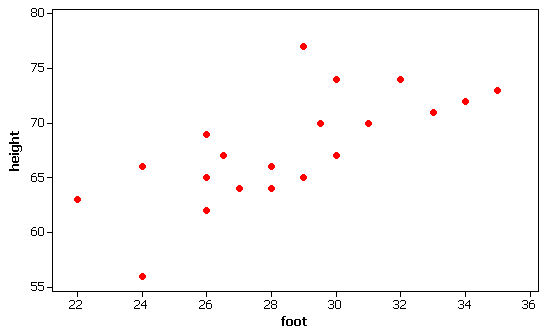
To see whether we can make better predictions of height by taking foot length into account, consider the following scatterplot of the height (in inches) and foot length (in centimeters) for the sample of 20 statistics students.
There is a fairly strong (\(r = 0.711\)), positive, linear association between height and footlength. As expected, people with larger (above average) feet tend to also be taller (above average height).
Use the Analyzing Two Quantitative Variables applet (below) to see the scatterplot of the 20 students’ height and foot measurements. Check the Show Movable Line box to add a blue line to the scatterplot. The equation for this initial line, \(\hat{height} = 67.75 + 0 \cdot footlength\text{,}\) predicts the same height for all 20 students as you did in Question 4. (Note: the “hat” over height indicates that the equation gives values for predicted height.)
If you now place your mouse over the green square on one of the ends of the line and drag, you can change the slope of the line. You can also use the mouse to move the green square in the middle of the line up and down vertically to change the intercept of the line.
Use good statistical notation, which means to use variables names (not generic \(x\) and \(y\)) and to put a “hat” over the response variable to indicate prediction.
Check the Show Residuals box to visually represent these residuals for your line on the scatterplot. The applet also reports the sum of the absolute residuals (or SAE, the sum of absolute errors).
Now check the Show Regression Line box to determine and display the equation for the line that actually does produce the smallest possible sum of squared residuals.
Report its equation and SSError value. Did everyone obtain the same line/equation this time? How does it compare to your line? (You can also display the residuals and the squared residuals for this line.)
The line that minimizes the sum of squared residuals is called the least squares line, or simply the regression line, or even the least squares regression line.
Suggest a technique for determining (based on the observed data \(x_i\)’s and \(y_i\)’s) the values of the slope and the intercept that minimize the SSError.
Least Squares Regression Line: Derivation of Coefficients.
The least squares line \(\hat{y} = b_0 + b_1 x\) is determined by finding the values of the coefficients \(b_0\) and \(b_1\) that minimize the sum of the squared residuals, \(SSError = \sum(y_i - \hat{y}_i)^2 = \sum_{i=1}^{n}(y_i - b_0 - b_1 x_i)^2\text{.}\)
Take the derivative with respect to \(b_0\) of the expression on the right. Then take the derivative of the original expression with respect to \(b_1\text{.}\)
Solve the first equation for \(b_0\text{.}\) Then solve the second equation for \(b_1\) (substituting in the expression for \(b_0\) using the summation notation).
With a little bit more algebra, you can show that the formulas for the least squares estimates of the intercept coefficient \(b_0\) and slope coefficient \(b_1\) simplify to:
For the sample data on students’ foot lengths (\(x\)) and heights (\(y\)), we can calculate these summary statistics: \(\bar{x} = 28.5\) cm, \(s_x = 3.45\) cm, \(\bar{y} = 67.75\) in and \(s_y = 5.00\) in, with \(r = 0.711\text{.}\) Use these statistics and the formulas above to calculate the coefficients of the least-squares regression line. Confirm that these agree with what the applet reported for the equation of the least squares line.
Use this least-squares regression line to predict the height of a person with a 28 cm foot length. Then repeat for a person with a 29-cm foot length. Calculate the difference in these two height predictions. Does this value look familiar? Explain.
The intercept is the predicted height for an individual whose foot length is zero, though it is not all that reasonable to predict someone’s height if their foot length is zero.
The slope coefficient of 1.03 indicates that the predicted height of a person increases by 1.03 inches for each additional centimeter of foot length. In other words, if one person’s foot length is one cm longer than another’s, we predict this person to be 1.03 inches taller than the other person. Notice we are being careful to talk about the “predicted” change or “average” change, because these are estimates based on the least squares line, not an exact mathematical relationship between height and foot length. The intercept coefficient can be interpreted as the predicted height for a person whose foot length is zero — not a very sensible prediction in this context. In fact, the intercept will often be too far outside the range of \(x\) values for us to seriously consider its interpretation.
Use the least squares regression line to predict the height of someone whose foot length is 44 cm. Explain why you should not be as comfortable making this prediction as the ones in Question 23.
The foot length of 44 cm is very far outside the range of the \(x\) values that were in the data set, so we might not be completely convinced the same relationship extends to such extreme values.
Extrapolation refers to making predictions outside the range of the explanatory variable values in the data set used to determine the regression line. It is generally ill-advised.
One way to assess the usefulness of this least-squares line is to measure the improvement in our predictions by using the least-squares line instead of the \(\bar{y}\) line that assumes no knowledge about the explanatory variable.
In the applet, uncheck and recheck the Show Movable Line box. Check the Show Squared Residuals box to determine the SSError if we were to use \(\bar{y}\) as our predicted value for every \(x\) (foot size).
The preceding expression indicates the reduction in the prediction errors from using the least squares line instead of the \(\bar{y}\) line. This is referred to as the coefficient of determination, interpreted as the percentage of the variability in the response variable that is explained by the least-squares regression line with the explanatory variable. This provides us with a measure of how accurate our predictions will be and is most useful for comparing different models (e.g., different choices of explanatory variable). The coefficient of determination is equal to the square of the correlation coefficient and so is denoted by \(r^2\) or \(R^2\) (and is often pronounced “r-squared”).
Another measure of the quality of the fit is \(s\text{,}\) the standard deviation of the residuals. This is a measure of the unexplained variability about the regression line and gives us an idea of how accurate our predictions should be (the actual response should be within \(2s\) of the predicted response). If \(s\) is much smaller than the variability in the response variable (\(s_y\)) then we have explained a good amount of variability in \(y\text{.}\) Most statistical packages report \(s\text{,}\) or it can be found from \(\sqrt{SSError/(n-2)}\text{.}\)
The observations tend to fall about 3.61 inches from the regression line. This is a typical prediction error. About 95% of the time we will be able to use this model to predict someone’s height within 7.2 inches. We have reduced the typical prediction error from about 5 inches to 3.61 inches.
There is a fairly strong positive linear association between the foot length of statistics students and their heights (\(r = 0.711\)). To predict heights from foot lengths, the least-squares regression line is \(\hat{height} = 38.3 + 1.03 \cdot foot\text{.}\) This indicates that if one person’s foot length measurement is one centimeter longer than another, we will predict that person’s height to be 1.03 inches taller. This regression line has a coefficient of determination of 50.6%, indicating that 50.6% of the variability in heights is explained by this least squares regression line with foot length. The other 49.4% of the variability in heights is explained by other factors (perhaps including gender) and also by natural variation. So although the foot lengths are informative, they will not allow us to perfectly predict the heights of the students in this sample. The value of \(s\) is 3.61 inches, meaning we should be able to predict a person’s height within 3.61 inches based only on the size of his or her foot.
To store the predicted values, select Save Predicteds. Note that this column is created and saved in your table using a Formula (view the equation for the regression line in the Formula box).