Section3.6Investigation 1.6: Kissing the Right Way
In the previous investigation, you learned how to decide whether a hypothesized value of the parameter is plausible based on a two-sided p-value. The two-sided p-value is used when you do not have a prior suspicion or interest in whether the hypothesized value is too large or too small. In fact, in many studies we may not even really have a hypothesized value, but are more interested in using the sample data to estimate the value of the parameter. What are all the plausible values for the parameter?
Most people are right-handed and even the right eye is dominant for most people. Researchers have long believed that late-stage human embryos tend to turn their heads to the right. German bio-psychologist Onur Güntürkün (Nature, 2003) conjectured that this tendency to turn to the right manifests itself in other ways as well, so he studied kissing couples to see whether both people tend to lean their heads to the right more often than to their left (and if so, how strong the tendency is).
He and his researchers observed couples from age 13 to 70 in public places such as airports, train stations, beaches, and parks in the United States, Germany, and Turkey. The observers were careful not to include couples who were holding objects such as luggage that might have affected which direction they turned. We will model the overall decision-making process when kissing as a binomial random process.
Dr. Güntürkün actually conjectured that 2/3 of kissing couples would lean right in the long run. A Tic-Tac ad once claimed 74% of kissing couples lean right. State appropriate null and alternative hypotheses for each conjecture.
Based on Dr. Güntürkün’s result, what is your best guess for \(\pi\text{,}\) the long-run probability a kissing couple leans right? Do you think 0.50 will be a plausible value for \(\pi\text{?}\) 2/3? 0.74? Explain your reasoning.
We could employ a "trial-and-error" type of approach to determine which values of \(\pi\) appear plausible based on what we observed in the sample. This involves testing different values of \(\pi\) and seeing whether the corresponding two-sided p-value is larger than some pre-specified cut-off, typically 0.05. (This cut-off is often called the level of significance.) That is, we will consider \(\pi_0\) a plausible value for \(\pi\) if assuming \(\pi = \pi_0\) does not make our sample statistic look surprising (yielding a small p-value).
For each value below, determine whether observing 80 of 124 successes yields a two-sided p-value greater than 0.05. Check all plausible values (p-value \(\geq\) 0.05):
Use the applet to find the exact two-sided p-value (using the tails of the binomial distribution) for each hypothesized value. Plausible values have p-values \(\geq\) 0.05.
What you found in the previous exercise will be called a "95% confidence interval" as it was derived using the \(1 - 0.95 = 0.05\) cut-off value/significance level.
Use the One Proportion Inference applet to determine the 99% confidence interval by using 0.01 rather than 0.05 as the criterion for rejection/plausibility (level of significance).
Using 0.01 as the significance level, test different values of \(\pi_0\) to determine which yield a two-sided p-value greater than 0.01. Check all plausible values (p-value \(\geq\) 0.01):
You can check the Show sliders box in the applet and use the slider or edit the orange number to change the value of \(\pi_0\text{.}\) Keep in mind that you are changing the conjectured value of \(\pi\text{,}\) not the observed number of successes, which should stay at 80.
Explanation: To be more confident (99% vs. 95%) that we’ve captured the true parameter value, we need to include more values, making the interval wider.
Identify a value that is captured in the 99% confidence interval but not the 95% confidence interval. Interpret the meaning of this observation. Explain what your analysis reveals about this value as a plausible value of \(\pi\text{.}\)
The researchers are assuming they have a representative sample from a binomial random process and want to estimate \(\pi\text{,}\) the underlying probability that a randomly selected kissing couple leans to the right. Based on this sample of 124 observations, we estimate \(\pi\) to be close to \(\hat{p} = 80/124 = 0.645\text{.}\) However, we know there is some sampling variability, so we want to find an interval of values that appear to be plausible values of \(\pi\text{.}\) We do this by finding the values of \(\pi_0\) for which the two-sided p-value (\(H_0\!:\pi = \pi_0\) vs. \(H_a\!:\pi \neq \pi_0\)) is greater than 0.05. These are all the values of the parameter such that our sample result is not overly surprising. You should have found this "95% confidence interval," using the "smallest tail probability" approach, to be approximately 0.557 to 0.727 (results from using different software or the applet will differ slightly). Thus, based on these sample results, we are "confident" that the actual value of \(\pi\text{,}\) the probability a random kissing couple leans right, is between 0.56 and 0.73.
A 99% confidence interval for \(\pi\) extends from 0.529 to 0.749 (a smaller lower endpoint and a larger upper endpoint, but a similar midpoint) and therefore includes additional plausible values of the parameter compared to the 95% interval. The 99% confidence interval is wider than the 95% interval because a higher level of confidence requires more "room for error." You will learn other methods for calculating confidence intervals for a binomial process in the next section.
In this investigation you have learned a second type of "statistical inference": providing an interval of plausible values for the parameter based on an observed sample statistic. Confidence intervals provide a nice companion to tests of significance and are also very useful by themselves. Whereas a test of significance allows you to test the plausibility of a specific hypothesized value, if you reject the null hypothesis, the test of significance provides no information as to how different the actual parameter is from the hypothesized value. If you fail to reject the null hypothesis, you only know that the tested value is one of many plausible values. A confidence interval provides an estimate (with bounds) of the actual value of the parameter. You will learn some additional methods for finding confidence intervals later in this text, but do be aware that some software packages use different methods for finding the "exact" binomial two-sided p-values.
Alternatively, another way to define a binomial confidence interval is to find all the values of \(\pi\) such that P(X < observed) < (1 – confidence level)/2 and P(X > observed) < (1 – confidence level)/2. Use the applet to find the 95% confidence interval using this approach. [Hints: Remember to use the one-sided p-value and change the direction of the tail probability between < and >, but not =.]
Neither is definitively "better" - they use different definitions of "more extreme." The Blaker method tends to produce slightly shorter intervals and is increasingly preferred.
Probability Detour – Binomial Confidence Intervals.
Probably the most well-known binomial confidence interval method is the Clopper-Pearson method (Biometrika, 1934). Rather than using two-sided p-values, it will consider a value for \(\pi\) plausible as long as the one-sided tail probability is smaller than (1 – confidence level)/2. One advantage of the Clopper-Pearson method is there is a simple computer algorithm for finding it, rather than needing to check all values as you have done here.
The method we first showed you (keeping all values of \(\pi\) with a two-sided p-value larger than (1 – confidence level) using the two-sided p-value based on the tail probabilities) is attributed to Blaker (The Canadian Journal of Statistics, 2000). We could refer to this as the "smallest tail probability" method.
Another approach would be to use the "smallest p-value" approach for the two-sided p-value, switching to using P(X = x) to find values of x more extreme than observed in finding the two-sided p-value. This method, attributed to Sterne (Biometrika, 1954), has the disadvantage that the interval produced can have holes! For example, a value like 0.12 may be in the interval of plausible values, the value 0.13 may not, and the value 0.14 may be again.
Many prefer the Blaker method to the holes of the Sterne method, and Blaker’s method is now gaining favor over Clopper-Pearson because the intervals tend to be shorter. We will see some other methods later in this text as well. For now, keep in mind the likely duality between confidence intervals and tests of significance: The confidence interval is the set of values for which we would fail to reject the null hypothesis in favor of the two-sided alternative. So we can interpret the confidence interval as the set of plausible values for the parameter in that they are the values such that our observed sample result would not be surprising. Keep in mind that saying a value is plausible is not the same as saying a value is probable. We won’t make probability statements about parameter values in this text.
The parameter \(\pi\) is a fixed value - it either is or isn’t in the interval. The 99% refers to the confidence in our method: if we were to repeat this process many times, about 99% of the intervals we construct would contain the true parameter value. We cannot make a probability statement about this specific interval containing the parameter.
Use technology to determine the 95% and 99% Clopper-Pearson confidence intervals for the probability that a kissing couple leans to the right. Comment on how the 99% confidence interval compares to the 95% interval, examining both midpoints and widths.
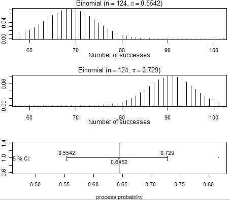
The bottom graph illustrates the 95% confidence interval. The interval is centered at the observed sample proportion \(\hat{p}\) and displays the two endpoints of the interval of plausible values for the process probability.
The top graph shows the distribution assuming the lower value of the confidence interval as the process probability. This is as far left as we can shift that null distribution before the area to the right of the observed number of successes, 80, dips below 0.025.
The middle graph shows how far we can move that distribution to the right (largest plausible value of \(\pi\)) before the probability below 80 dips below 0.025.
Based on this result, what is an interval of plausible values for the underlying mortality rate at St. George’s? [Hint: You can use a 95% confidence level if none is stated.] Describe how you found the interval and name the method used. Report the midpoint and width of this interval.
Use technology to calculate the 95% confidence interval based on the 71 deaths among 361 patients. Comment on how the width and midpoint of this interval differ from the interval in the previous question. Explain why these changes make sense.
Based on the interval in the previous question, if you were to test \(H_0\!:\pi = 0.20\) vs. \(H_a\!:\pi \neq 0.20\text{,}\) would you reject or fail to reject the null hypothesis? Explain how you know the conclusion based on the confidence interval without actually conducting the test.