Excel Exploration: Minimization Criteria

Section 26.6 Excel Exploration: Minimization Criteria

Exercises Exploration Tasks

Another way to get around the problem revealed in Question 7 and Question 8 of Investigation 5.8, that the sum of residuals from the mean always equals zero, is to examine the sum of the absolute deviations.

1. Compute SAE from Mean.

Using your results in the table in Question 4 of Investigation 5.8, calculate the sum of the absolute values of the residuals, using the mean height as the predicted value.

Solution.

\(SAE = 80.5\)

Let’s investigate whether there is a better number (call it \(m\)) than the mean to use for predicting height, in order to minimize our prediction errors. In general, this sum of absolute residuals (or SAE, sum of absolute errors) can be written:

\begin{equation*} SAE = \sum_{i=1}^{n} |y_i - m| \end{equation*}

The problem with using the SAE is that it is not easily differentiable, so we cannot use calculus to determine the optimal value for \(m\text{.}\) Instead, we will use Excel to explore the behavior of SAE as a function of \(m\text{.}\) We will look for the value of \(m\) that minimizes SAE.

Open the Excel spreadsheet document Heights.xls. Notice that the 20 heights are in column A (sorted), and column B contains candidates for \(m\) from 65 to 70, in increments of 0.01.
Click on cell C2, and notice that it contains a formula for SAE(\(m\)), which refers to the data values in column A and to the value of \(m\) from B2 (namely, \(m = 65\) in that cell).
Use Excel’s “fill down” feature to calculate the values of \(SAE(m)\) for the remainder of column C. [Hint: You can do this in one of several ways: With the C2 cell selected, double click on the box in the lower right corner, or pull the right corner of the highlighted C2 cell down to the end of the column, or highlight C2 and the cells to be filled and choose Edit > Fill > Down.]

2. Compute SAE(m) in Spreadsheet.

Confirm that the SAE value for the sample mean (67.75) agrees with what you calculated in Question 1.

Yes, the spreadsheet’s SAE value for \(m = 67.75\) agrees with my calculation.
Good — both should give \(SAE = 80.5\text{.}\)
No, the two values do not agree.
Recheck your calculation in Question 1 (and make sure you are looking at the row for \(m = 67.75\)); both should give \(SAE = 80.5\text{.}\)

Solution.

Excel columns B and C with the row m = 67.75, SAE = 80.5 highlighted.

To produce a graph of SAE as a function of \(m\text{:}\)

Highlight columns B and C. Choose Insert > Scatter and then choose the first option in the second row (Scatter with Smooth Lines) to construct a graph of this function.

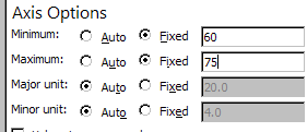
Excel Insert ribbon Scatter chart menu with the Scatter with Smooth Lines option highlighted.

Excel Format Axis dialog with the horizontal axis Minimum fixed at 60 and Maximum fixed at 75.

[Hint: After you create the graph, you may want to change the x-min and x-max values by double clicking on the horizontal axis and changing the Minimum and Maximum under Axis Options.]

3. Graph SAE(m).

Comment on the shape of this function. Does it seem to follow a familiar form, such as linear or parabolic or exponential? Explain.

Solution.

Excel graph of SAE versus m from 64 to 71: a piecewise-linear V shape with its minimum near m = 67, SAE = 79.

Excel columns B and C with the row m = 67, SAE = 79 highlighted.

It looks like a piecewise parabola.

4. Find Minimizer of SAE.

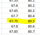
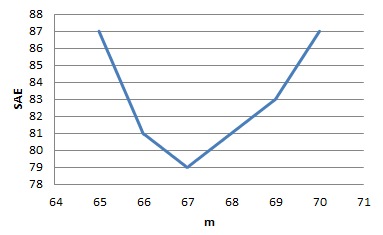
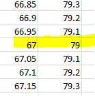
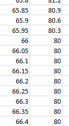
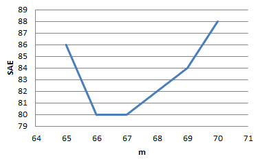
Does there seem to be a unique value of \(m\) that minimizes this SAE(\(m\)) function? If so, identify it. If not, describe all values of \(m\) that minimize the function. Also report the value of the SAE for this optimal value of \(m\text{.}\)

Hint.

Search through the entries in column C to find the smallest value, and then read off the corresponding value in column B.

Solution.

The function appears to be minimized at 67 in, with an SAE value around 79.

5. Connect to Median.

Look through the sorted heights in column A. What do you notice about where this optimal value of \(m\) is located in the list of sorted heights? Does this remind you of a familiar statistic?

Solution.

There are 20 observations and 67 is the 10th (and 11th) value. An observation falling between the 10th and 11th observations is the median of the 20 values.

Suppose the tenth largest height (in row 11) had been 66 inches instead of 67. Make this change to the spreadsheet (cell A11), and note that the graph of the SAE function is updated automatically.

6. Modify Middle Value.

Now is there a unique value of \(m\) that minimizes this SAE(\(m\)) function? If so, identify it. If not, describe all values of \(m\) that minimize the function, and also report the (optimal, minimum) value of the SAE.

Solution.

Excel columns B and C showing SAE equal to 80 for every value of m from 66 to 66.4.

Excel graph of SAE versus m with a flat bottom: SAE stays at 80 for all m between 66 and 67.

This creates a flat spot in the graph. Now all values between 66 and 67 (inclusive) minimize the SAE at 80.

Return the tenth largest height back to 67 inches. Now suppose the tallest person in the sample had been 80 inches tall instead of 77. Make this change to the spreadsheet (cell A21)

7. Modify Extreme Value.

Describe how the graph of the SAE function changes. Also report the value of the SAE.

Solution.

This just moves the graph up (with the same shape) to higher SAE values. The optimal \(m\) is still 67 with an SAE value of 82.

8. General Conjecture.

Based on these findings, make a conjecture as to how one can determine, from a generic set of 20 data values, the value that minimizes the sum of the absolute prediction errors from the data values.

Solution.

The median (or any value between the 10th and 11th sorted values).

Consider a new minimization criterion: mean absolute error (MAE) criterion, which divides the SAE value by the number of observations.

9. MAE Criterion.

How would the MAE(\(m\)) function compare to the SAE(\(m\)) function? Would its minimum be achieved at the same value(s) of \(m\text{?}\) Explain.

Solution.

The values of the SAE would change, again proportionally, and the optimal \(m\) would remain the same.

Discussion.

You should have found that the SAE function is piecewise linear. In other words, the function itself is not linear, but its component pieces are linear. In this case the function changes its slope precisely at the data values. The SAE function (and MAE function) are minimized at the median of the data and also at any value between (and including) the two middle values in the dataset (the 10th and 11th values in this case with \(n = 20\) values). It is a convenient convention to define the median as the average (midpoint) of those two middle values. The MAE has a bit more natural interpretation — the average deviation of the values in the data set from the value of \(m\text{.}\)

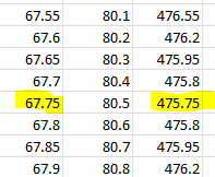
Another criterion is to find the value of \(m\) that minimizes the sum of the squared deviations.

10. Least-Squares Minimizer Recall.

Recall from Question 10 of Investigation 5.8 the value of \(m\) that minimizes the sum of the squared prediction errors. Report this value of \(m\) for the height data.

Solution.

This was the mean, here 67.75 in.

Make sure that the data values in column A are back to their original values. Then click on cell D2 in the Excel spreadsheet, and notice that it gives the formula for the SSE (sum of squared errors) function.
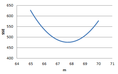
Fill this formula down the column and create a second graph to display the behavior of this function. [Hints: Click on column B and then hold the mouse down when you click on column D to highlight just those two columns before you insert the graph. You will probably want to double click on the y-axis scale to change its minimum value.]

11. Graph SSE(m).

Does this function have a recognizable form, such as a polynomial? What is its shape? At what value of \(m\) is the function minimized? Does this value look familiar?

Solution.

Excel graph of SSE versus m: a smooth parabola with its minimum near m = 67.75, SSE about 476.

Excel columns B, C, and D with the row m = 67.75, SAE = 80.5, SSE = 475.75 highlighted.

This is now a parabola, minimized at \(m = 67.75\) in (the sample mean) with an SSE value of 475.75.

12. Outlier Sensitivity Comparison.

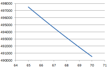
Suppose there had been a clerical error in entering the height of the tallest student. Change the height of the tallest student from 77 inches to 770 and investigate the effect on the SSE function. Has the value of \(m\) that minimizes SSE changed? By how much? How does this compare to the effect of this clerical error on the SAE function and where it is minimized?

Solution.

Excel graph of SSE versus m after changing 77 to 770: a steadily decreasing line from about 497,500 down to 490,500 with no minimum visible in the window.

This changes the function quite a bit and the optimal \(m\) is no longer displayed in the graph.

Discussion.

Although the SAE criteria would be more resistant to outliers, it does not always lead to a unique minimum (e.g., an even number of data values where the values of the middle pair are not equal). This has led to the more common criterion of least squares.

See the exercises for investigating additional minimization criteria, such as the median of absolute errors and maximum of absolute errors.

You have attempted of activities on this page.

Prev Top Next