Section 10.3 Investigation 2.9: Heroin Treatment Times

Exercises 10.3.1 The Study

Rabe-Hesketh and Everitt (2000) report on a study by Caplehorn and Bell (1991) that investigated the times that heroin addicts remained in a clinic for methadone maintenance treatment. The data in heroin.txt includes the amount of time that the subjects stayed in the facility until treatment was terminated (times, number of days). For about 37% of subjects, the study ended while they were still in the clinic (status = 0). Thus, their β€œsurvival time” has been β€œtruncated.” For this reason, we might not want to focus on the mean survival time, but rather some other measure of a β€œtypical” survival time. We will explore both the median and the 75th percentile. We will treat this group of 238 patients as representative of the population of heroin addicts.

1. Describe the survival times.

Produce and describe a histogram of the survival times for these patients.
Hint. R Hint
We will just focus on the times data, so you can copy and load all the data and then let
times = heroin$times
Solution.
The distribution of treatment times is skewed to the right, ranging from about 0 to 1000 days with a mean 402.6 days and median 367.5 days.
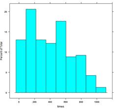
described in detail following the image
Histogram of survival times, skewed to the right, ranging from about 0 to 1000 days
2. Consider a mathematical model.

Explain why it is not likely that we could find a simple mathematical model for the distribution of this variable.
Solution.
The data do not appear to be unimodal. The models we have looked at so far (e.g., exponential, log normal) have all been unimodal. We also have to worry about the data having been truncated.

Bootstrapping.

Even though a sample size of \(n = 238\) is likely large enough for us to employ the Central Limit Theorem for the distribution of the sample mean, we may be more interested in the median or another statistic like a β€œtrimmed mean.” However, we may not know a mathematical model for the sampling distribution of one of these other statistics. Of course, what we are most interested in is a measure of the sample-to-sample variability of that statistic. Previously, we estimated the standard error of the sample mean by using information from the sample (\(s/\sqrt{n}\)). But when such a formula does not exist, another method that is gaining in popularity is bootstrapping.
Definition: Bootstrap Sample.
A bootstrap sample resamples the data from the existing sample, drawing the same number of observations, but with replacement. A bootstrap distribution is a collection of values of the statistic from lots of bootstrap samples.
The reasoning behind this technique is that if the sample has been randomly selected, it should be representative of the population. Thus, it should give us information about the population and about samples drawn from that population. In other words, rather than assume a particular probability model for the population, bootstrapping assumes that the population looks just like the sample, replicated infinitely many times. By sampling with replacement from the original sample, and calculating the statistics of interest for each bootstrap sample, we gain information about the shape and spread of the sampling distribution of the statistic of interest.
Key Result.
The plug-in principle states that the standard deviation of the bootstrap distribution provides a reasonable estimate of the standard deviation of the sampling distribution of the statistic.
Use technology to take a bootstrap sample from the heroin data.
Hint 1. Applet Instructions
In Sampling From Population applet: Follow the link for the Bootstrapping variation. Paste in the data and select the times variable. Check Show Sampling Options and set the Sample size to 238. Press Draw Samples. Set the Statistic radio button to Median.
Hint 2. R Instructions
sample1 = sample(x=times, size=238, replace = TRUE)
Hint 3. JMP Instructions
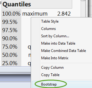
In the Analyze > Distribution output, in the Quantiles section, right click, and from the pop up menu select Bootstrap. Set the Number of Bootstrap Samples to one and press OK. This will open a new data window with the statistics from the bootstrap sample.
described in detail following the image
JMP Quantiles output with right-click menu showing the Bootstrap option circled
4. Take another bootstrap sample.
Take another bootstrap sample. Did you get the same bootstrap sample median? Why or why not?
Solution.
Results will vary, but highly unlikely you will get exactly the same sample median. Even though we are sampling 238 observations both times, because we are sampling with replacement, each sample consists of slightly different values, some repeating more than others, some not appearing.
To estimate the sample-to-sample variation in our statistic (e.g., the median), we now want to repeat this process a large number of times.
Hint 1. Applet Instructions
In Sampling From Population/Bootstrapping applet: Set the Number of samples to at least 998. Press Draw Samples.
Hint 2. R Instructions
Create a list of bootstrap samples and then apply the median to each sample:
resamples =lapply(1:1000, function(i) sample(times, 238,replace=T))
bootstrapmedians = sapply(resamples, median)
          
Hint 3. JMP Instructions
  • Set the number of bootstrap samples to 1000.
  • Then find the output of the 1000 bootstrap sample medians and copy and paste those into a new data table.
5. Create a bootstrap distribution.
Use technology to create a bootstrap distribution from the heroin data.
Solution.
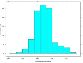
R output:
described in detail following the image
Histogram of 1000 bootstrap medians from R, roughly symmetric and centered near 375
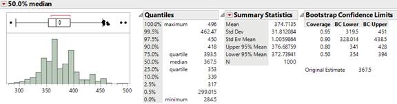
JMP output:
described in detail following the image
JMP bootstrap output for the median: histogram, quantiles, summary statistics, and bootstrap confidence limits
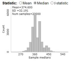
Applet output:
described in detail following the image
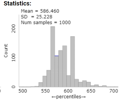
Applet histogram of sample medians with mean 374.600 and SD 32.191
You should now have a collection of the medians from 1000 different bootstrap samples.
6. Describe the bootstrap distribution.
Produce graphical and numerical summaries of the 1000 bootstrap medians. Describe the behavior of the bootstrap distribution.
Solution.
The distribution is pretty symmetric, centered around 375 days, with standard deviation around 32 days (results will vary).
7. Calculate a rough confidence interval.
Suggest a quick method for using the distribution in Question 5 to calculate a rough confidence interval for the population median. Calculate and interpret this interval.
Hint.
Recall our usual estimate \(\pm\) 2 \(\times\) standard deviation of estimate.
Solution.
We could take the observed sample median (367.5) and add and subtract two SD(medians) \(\approx\) 32.
For example 367.5 \(\pm\) 2(32) = (303.5, 431.5)
We are 95% confident that the median treatment time in this population is between 303.5 and 431.5 days.
Discussion.
Once you get an estimate of the standard deviation of the statistic, there is still some consideration of how to construct a confidence interval. In this case, the distribution of medians should look fairly symmetric, so a symmetric confidence interval can work. In other cases, there are more complicated β€œadjustments” that can be made to get a bootstrap confidence interval. Discussion of these methods is beyond of the scope of this text, but you have seen an example of the power of bootstrapping β€” you can create a distribution for any statistic that should have the same variability as the sampling distribution of that statistic, without having to pretend you know anything about the population!
Repeat this analysis, but now using the upper quartile (75% percentile) as the statistic.
Hint 1. Applet Instructions
Select the Percentile radio button. Enter .75 in the box that appears and press Draw Samples.
Hint 2. R Instructions
quantile(heroin$times, c(.75))
bootstrap75th <- sapply(resamples, quantile, p=.75)
          
Hint 3. JMP Instructions
Return to the earlier data window and select the bootstrap results for the 75.0% quartile.
8. Bootstrap the upper quartile.
Interpret your results.
Solution.
In R, observed 585.5
resamples <- lapply(1:1000, function(i) sample(times, 238, replace=T))
bootstrapmedians <- sapply(resamples, quantile, p = .75)
iscamsummary(bootstrapmedians)
        
585.5 \(\pm\) 2*25.19, 585.5 \(\pm\) 2*25.19 \(\approx\) (535.1, 635.9)
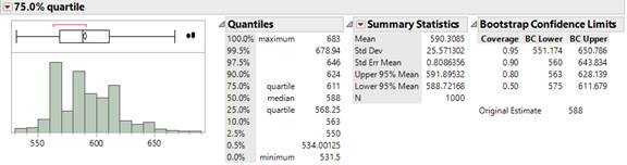
In JMP, observed = 588
described in detail following the image
JMP bootstrap output for the 75% quartile: histogram, quantiles, summary statistics, and bootstrap confidence limits
588 \(\pm\) 2(25.57) = (536.9, 639.1), though distribution is not very symmetric
In applet, observed = 584
described in detail following the image
Applet histogram of bootstrap 75th percentiles with mean 586.460 and SD 25.228
585 \(\pm\) 2(25.228) = (534.5, 635.5)

Study Conclusions.

The distribution of treatment times was skewed to the right with a median of about 1 year (367.5 days) and interquartile range of 418.5 days. Because of the skewness and truncation in the data, we might prefer the median or even the third quartile as the statistic. Based on a bootstrap simulation, an approximate 95% confidence interval for the median treatment time in the population of heroin addicts is between 306 days and 430 days (but results will vary), while an approximate 95% confidence interval for the upper quartile is around 534 to 638 days (results will vary). The interval for the median includes lower values than a t-interval for the population mean (368, 437), because the t-procedure is more strongly affected by the skewness in the data. We would like to generalize these data to all heroin patients, but would like more information to ensure this sample is representative.

Subsection 10.3.2 Practice Problem 2.9A

In April 2014, the city of Flint Michigan switched its water supply to the Flint River in an effort to save money. The U.S. Environmental Protection Agency (EPA)’s Lead and Copper Rule states that if lead concentrations exceed an action level of 15 parts per billion (ppb) in more than 10% of homes sampled, then actions must be undertaken to control corrosion, and the public must be informed. Consider the data in flint_mdeq.txt

Checkpoint 10.3.7. Bootstrap interval for the 90th percentile.

Create a bootstrap confidence interval for the 90th percentile using the full dataset (\(n = 71\)). Describe your approach in detail.
After the city submitted their data, the state instructed them to drop two of the values because they violated testing guidelines. One measurement was dropped because there was a water filter in the home β€” which could give an artificially low measurement β€” but actually this value was 104 ppb, the maximum by far. The other dropped value, 20 ppb, also on the high side, was dropped because it came from a business, not a home.

Checkpoint 10.3.8. Compare after removing observations.

Create a bootstrap confidence interval after removing the two questionable observations (\(n = 69\)). How do the results compare?

Subsection 10.3.3 Practice Problem 2.9B

Return to the honking.txt data from Investigation 2.2.

Checkpoint 10.3.9. Consider the Central Limit Theorem.

Suggest a reason why the Central Limit Theorem may not apply with these data.

Checkpoint 10.3.10. Bootstrap interval for the median.

Create and interpret an informal (\(\pm\) 2SE) bootstrap confidence interval for the population median.
You have attempted of activities on this page.