A physical education teacher at a junior high school in Central California wanted to determine whether there is a relationship between seventh-graders’ times to run a mile and how many push-ups they can do under controlled conditions. She collected the data in PEClass.txt as part of the mandated state physical fitness testing program. Analyze these data to address the question of whether they provide evidence of a relationship between these two variables. Include graphical and numerical summaries as well as a test of significance. Summarize your conclusions.
Solution.
Because we have two quantitative variables here (time to run one mile and number of push-ups), the appropriate analysis would be regression. We first want to examine numerical and graphical summaries. When you open
PEClass you will notice that the mile run times have been recorded in “time format.” We want to convert this to numerical values. For example, in R (R is going to assume you have hr: min)
> miletimeformat = as.POSIXlt(paste(Sys.Date(), peclass$MileTime))
> miletimes = miletimeformat$hour + miletimeformat$min/60
In JMP, use Cols > Column Info. In two steps, first change the Data Type to Numeric and the Modeling Type to Continuous and then select the Format as Duration, min: s. For the second step, again choose Cols > Column Info, and this time just change the Format to Best. Then divide by 60. Now you should have the number of minutes (including the fraction of minute) for each student. (Your first result should be 11.917 min.)
Because we aren’t considering either of these as a response variable, it does not matter which variable we denote as the y-variable and which as the x-variable. If we plot mile time vs. push-ups, we see there is a strong negative association.
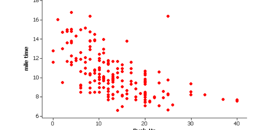
Scatterplot of mile time (minutes) versus push-ups showing a strong negative association: students completing more push-ups tend to have faster mile times.
Students who do more push-ups also tend to run the mile in faster times. However, there is some evidence that the relationship is not linear. There is also an unusual observation, a student who did a larger number of push-ups but was one of the slowest runners. Carrying out the regression and examining residual plots confirms these observations.
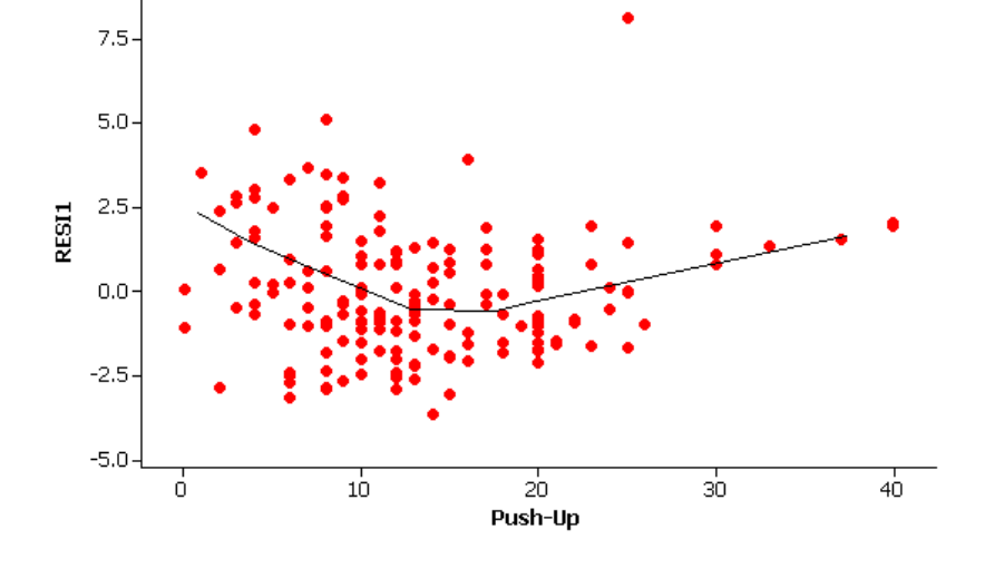
Plot of residuals (RESI1) versus push-ups with a curved smoother: residuals are positive at the low and high ends of push-ups and negative in the middle, suggesting curvature, plus one large positive outlier.
The residual vs. explanatory variable graph also reveals some differences in the amount of variation in the residuals at different values of the explanatory variable (indicating a violation of the constant variance condition).
It appears that transforming these data might be helpful. Because both distributions appear skewed to the right (if you looked at histograms of each variable individually), we could consider taking the log of each variable. The log-log scatterplot does appear more well behaved. (We have used log base ten but natural logs would also work.)
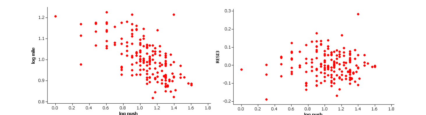
Two plots: a scatterplot of log mile versus log push showing a more linear negative association, and a plot of the residuals (RESI3) versus log push showing random scatter around zero.
We still have some outliers but appear to now have a linear relationship. If we also examine the normality of the residuals:
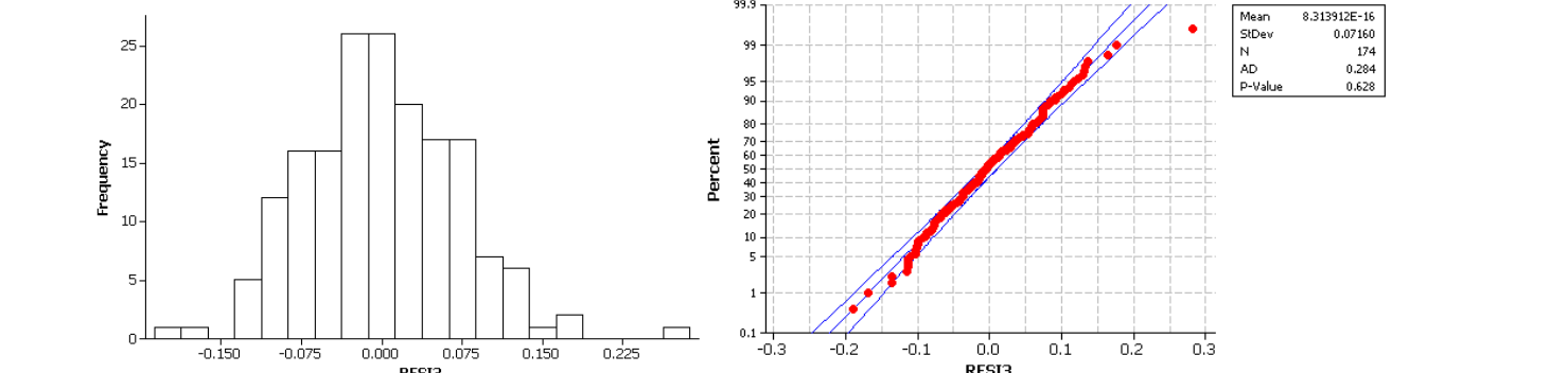
Histogram of the residuals (RESI3), roughly symmetric and centered at zero, and a normal probability plot with the points following the line closely; the legend reports mean essentially zero, SD 0.0716, n 174, AD 0.284, p-value 0.628.
This condition also seems to be reasonably met for the transformed data. There is slight evidence of skewness to the right in the residuals but coupled with the large sample size we will not be concerned with this minor deviation.
The correlation coefficient for the transformed variables is \(-0.624\text{,}\) indicating a moderately strong negative linear relationship between log(time) and log(push-ups). The least-squares regression equation is computed by Minitab to be \(\log\hat{mile} = 1.23 - 0.213\,\log(\text{push-ups})\text{.}\) The intercept coefficient here would indicate the predicted log-time for a student who only completes 1 push up (so log(push-ups) = 0) to be 1.23. This corresponds to a time of \(10^{1.23}\) or about 17 minutes. The slope coefficient predicts the average multiplicative change in the log-mile times for each unit increase in log(push-ups). A unit increase in “log(push-ups)” corresponds to the push-ups increasing by a factor of 10. So for each 10 fold increase in the number of push-ups (e.g., 1 push up to 10 push-ups), the mile time decreases on average by a factor of \(10^{-.213} = 0.61\text{.}\) [Note: our prediction for 10 push-ups is 1.017, corresponding to \(10^{1.017} \approx 10.4\) minutes, which is 0.61(17).]
If we test the significance of this correlation:
Let \(\beta\) represent the true population slope between log(time) and log(push-ups)
\(H_0\text{:}\) \(\beta = 0\) (there is no association between these two variables)
\(H_a\text{:}\) \(\beta \neq 0\) (there is an association)
We find a standardized statistic of \(t = -10.48\) and a two-sided p-value of approximately 0.
Predictor       Coef  SE Coef       T      P
Constant     1.24825  0.02218   56.28  0.000
log push    -0.21315  0.02033  -10.48  0.000
Note: This p-value is the same as with the sample correlation coefficient.
With such a small p-value (\(\lt 0.001\)) we would consider the relationship between log(time) and log(push-ups) to be statistically significant. Although we need to have some caution in generalizing these results to other schools, we can eliminate “random chance” as an explanation for the strong log-log relationship observed in this sample.
If we wanted to use this model to carry out predictions, we need to keep the transformed nature of the variables in mind. For example, if a student completed 25 push-ups during that portion of the test, we would predict \(1.23 - 0.213\,\log_{10}(25) = 0.932\) for the log-time and therefore \(10^{.932} = 8.56\) minutes for the mile time. We also need to start being a little cautious in predicting the mile time for such a large number of push-ups as we do not have a large amount of data in this region and our estimate will not be as precise.
In summary, there is a strong negative relationship between number of push-ups and time to run a mile for these 7th and 8th graders as we would expect (those students who do more than the average number of push-ups will tend to be the same students who complete a mile faster, in a below average time). This relationship can be considered statistically significant after performing log transformations, however, we have to be cautious in generalizing these results beyond this sample as the students were not randomly selected from a larger population of junior high students. Because this is an observational study, we are not claiming that doing more push-ups will cause the mile time to decrease.
We also saw in an earlier example that there was a statistically significant difference between males and females on these tasks and we might want to consider incorporating that variable into our analysis as well. For example, a coded scatterplot shows that the males tended to do more push-ups and also tended to be slightly faster than females on the mile times.
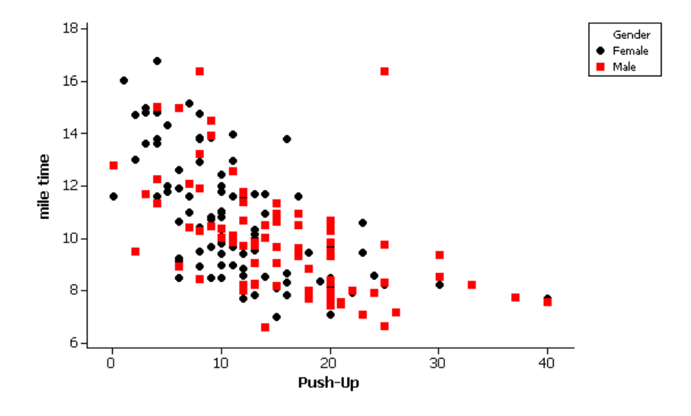
Coded scatterplot of mile time versus push-ups with females as black circles and males as red squares; the males tend to appear at higher push-up counts and slightly faster mile times.
We can actually carry out a multiple regression analysis to predict mile time from both push ups and gender.
Coefficients

Term            Coef    SE Coef        T      P
Constant    0.529616  0.0125671  42.1430  0.000
Push-Up    -0.007340  0.0008250  -8.8977  0.000
Gender
  Female    0.000481  0.0061047   0.0788  0.937
This analysis reveals that push-ups are strongly related to mile times even after adjusting for gender (meaning this association is strong among the females and also among the males), but if you know the someone’s push-up count, it is not that valuable to also know their gender.

