Section 26.1 Investigation 5.6: Cat Jumping

Exercises 26.1.1 The Study

Evolutionary biologists are often interested in β€œform-function relationships” to help explain evolution history of say an animal species. Harris and Steudel (2002) investigated factors that are related to the jumping ability of domestic cats.
Because jump ability and height are largely dependent on takeoff velocity, several traits were recorded for 18 healthy adult cats such as relative limb length, relative extensor muscle mass, body mass, fat mass relative to lean body mass, and the percentage of fast-twitch muscle fibers to see which might best explain maximum takeoff velocity (based on high-speed videos).
In this investigation, you will examine the following data, also available in the file CatJumping.txt:
ID Sex Body mass (g) Hind limb length (cm) Muscle mass (g) Percent body fat Takeoff velocity (cm/sec)
A F 3640 29.1 51.15 29 334.5
B F 2670 28.55 46.05 17 387.3
C M 5600 31.74 95.9 31 410.8
D F 4130 26.9 55.65 39 318.6
E F 3020 26.11 57.2 15 368.7
F F 2660 26.69 48.67 11 358.8
G F 3240 26.74 64.55 21 344.6
H M 5140 27.71 78.8 35 324.6
I F 3690 25.47 54.6 33 301.4
J F 3620 28.18 55.5 15 331.8
K F 5310 28.45 68.8 42 312.6
L M 5560 28.65 79.8 37 316.8
M M 3970 29.82 69.4 20 375.6
N F 3770 26.66 60.25 26 372.4
O F 5100 27.84 60.7 41 314.3
P F 2950 27.89 55.65 25 367.5
Q M 7930 30.58 98.95 48 286.3
R F 3550 28.06 79.25 16 352.5

Collecting the Data.

1. Identify Units and Response.
Identify the observational units and the primary response variable of interest here. Also classify this variable as quantitative or categorical.
Solution.
The observational units are the 18 cats and the primary response variable is takeoff velocity which is quantitative.
2. Univariate Summary of Velocity.
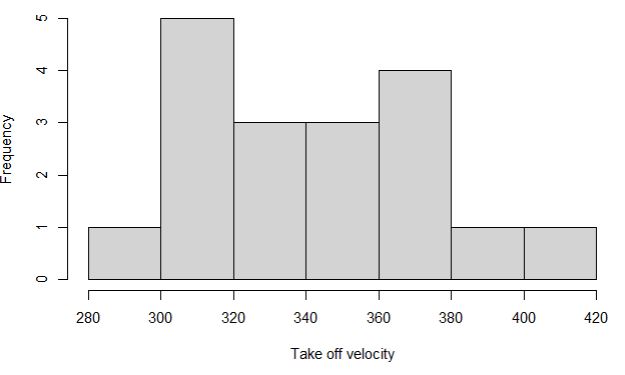
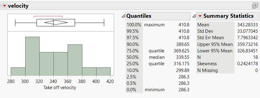
Open the CatJumping.txt data file and produce numerical and graphical summaries of the takeoff velocity variable. Describe the distribution of takeoff velocities in this sample (shape, center, variability, unusual observations).
Solution.
JMP output:
described in detail following the image
JMP output for velocity: boxplot and histogram of takeoff velocity from 280 to 420 cm/sec, with Quantiles (median 339.55, quartiles 316.175 and 369.625, maximum 410.8, minimum 286.3) and Summary Statistics (mean 343.28, standard deviation 33.08, n = 18).
R output:
described in detail following the image
R iscamsummary output for cats velocity: n = 18, minimum 286.3, Q1 317.25, median 339.55, Q3 368.4, maximum 410.8, mean 343.28, SD 33.077, skewness 0.222.
described in detail following the image
R histogram of takeoff velocity with bins from 280 to 420 cm/sec; tallest bar between 300 and 320, roughly mound-shaped with single observations in the 280, 380, and 400 bins.
The distribution is pretty symmetric or slightly skewed to the right (though depending on bin choices might see a visual outlier in the 420 bin). Most cats had a velocity around 320-380 cm/sec but one was as small as 286.30 cm/sec and the high outlier was at 410.80 cm/sec.
Note: 300 cm/sec corresponds to about 6.7 miles per hour.
3. Single-Value Prediction.
Based on your analysis of takeoff velocity, if you were going to randomly select a domestic cat, what is your best prediction of its takeoff velocity?
Solution.
Might pick the mean of 343.28 cm/sec.
4. Body Mass Conjecture.
Do you think there will be a relationship between a cat’s takeoff velocity and its body mass? If so, do you think heavier cats will tend to have larger or smaller takeoff velocities than lighter cats?
Solution.
Heavier cats might tend to have lower velocities.
We will need a new graphical summary to visually explore the relationship between two quantitative variables, the scatterplot.

Technology Detour: Scatterplots.

5. Scatterplot Instructions.
Hint 1. Applet Instructions
Hint 2. R Instructions
plot(bodymass, velocity) or plot(velocity~bodymass)
scatterplot(bodymass, velocity) (the scatterplot function is in the car package)
Hint 3. JMP Instructions
Solution.
JMP output:
described in detail following the image
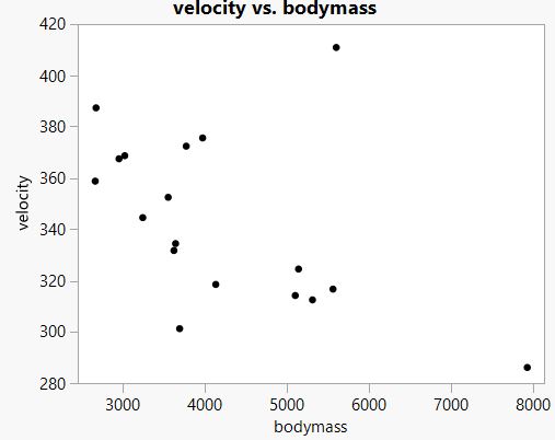
JMP scatterplot of velocity versus bodymass for the 18 cats, showing a negative association with one high-velocity outlier near bodymass 5600.
R output:
described in detail following the image
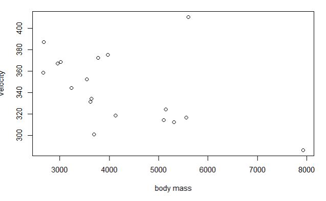
R scatterplot of velocity versus body mass showing the same negative association with the high-velocity outlier.
6. Describe Body Mass Relationship.
Describe the relationship between a cat’s takeoff velocity and its body mass, as displayed in this scatterplot. Does this pattern confirm your earlier expectation?
Solution.
Overall, heavier cats tend to have lower velocity (though one of the heaviest cats had the largest velocity).
7. Identify Outlier Cats.
Do any of these cats appear to be outliers in the sense that its pair of values (body mass, takeoff velocity) does not fit the pattern of the majority of cats? If so, identify the ID for that cat and describe what’s different about this cat (in context).
Solution.
ID: C
This cat has a much larger velocity than we would expect overall and for its weight.
Terminology Detour.
Scatterplots are useful for displaying the relationship between two quantitative variables. If one variable has been defined as the response variable and the other as the explanatory variable, we will put the response variable on the vertical axis and the explanatory variable along the horizontal axis.
In describing scatterplots you will describe the overall pattern between the two variables focusing primarily on three things:
  • Direction: Is there a positive association (small values of y tend to occur with small values of x and large values of y tend to occur with large values of x) or a negative association (small values of y tend to occur at large values of x and vice versa)?
  • Linearity: Is the overall pattern in the scatterplot linear or not?
  • Strength: How closely are the observations following the observed pattern?
The above scatterplot reveals a fairly strong, negative association between body mass and takeoff velocity, meaning that heavier cats tend to have a smaller takeoff velocity than larger cats. The relationship is somewhat linear but has a bit of a curved pattern. There is one outlier cat (cat C) with a very high takeoff velocity despite having a very large body mass.
8. Percent Body Fat Relationship.
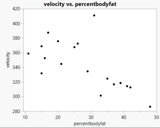
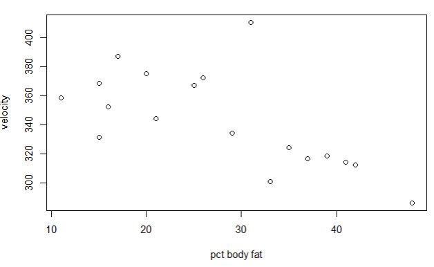
Now produce a scatterplot of takeoff velocity vs. percentage of body fat. Describe the association. Would you say that the association with velocity is stronger than with body mass? More or less linear?
Solution.
JMP output:
described in detail following the image
JMP scatterplot of velocity versus percentbodyfat showing a negative association with the same high-velocity outlier near 31 percent body fat.
R output:
described in detail following the image
R scatterplot of velocity versus percent body fat showing the same negative association with the high-velocity outlier.
This also appears to be an overall trend of cats with higher body fat percentages having lower velocities on average, except for our same outlier.
9. Other Predictors.
For the other two variables (hind limb length and muscle mass), would you expect to see a positive or negative association with takeoff velocity? Explain. Then look at scatterplots, and comment on whether the association is as you expected.
Solution.
conjectures will vary.
Muscle mass doesn’t appear to have as clear of a pattern but more muscle mass tends to have lower velocities.
Larger hind limb lengths tend to have larger velocities.

Technology Detour: Coded Scatterplots.

10. Coded Scatterplot Instructions.
Use technology to create a coded scatterplot of takeoff velocity vs. body mass that uses different symbols for male and female cats.
Hint 1. Applet Instructions
Hint 2. R Instructions
Create the scatterplot as before, but pass a categorical variable as a color vector. For example: plot(velocity~bodymass, col=sex)
Hint 3. JMP Instructions
Solution.
JMP output:
described in detail following the image
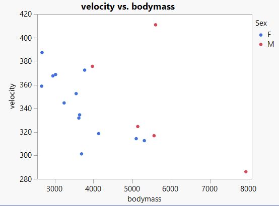
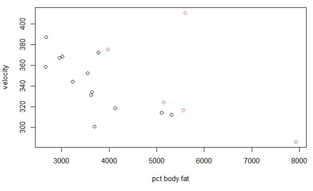
JMP coded scatterplot of velocity versus bodymass with a Sex row legend: female cats in blue, male cats in red; the males tend to be heavier.
R output:
described in detail following the image
R coded scatterplot of velocity versus body mass with points colored by sex; the male cats appear at the larger body masses.
11. Coded Scatterplot by Sex.
Based on this graph, do you notice any differences between male and female cats with regard to these variables? Explain.
Solution.
There are only 5 males but they tend to be heavier than the females. When the body mass is similar the velocities are similar though a little higher for males. The larger outlier is a male and there is also a very large male in terms of body mass.

Study Conclusions.

The researchers found significant relationships of takeoff velocity with hind limb length and fat-mass ratio, but not with all measured muscle variables. Later in this chapter you will study inferential tools for assessing these relationships.

Subsection 26.1.2 Practice Problem 5.6

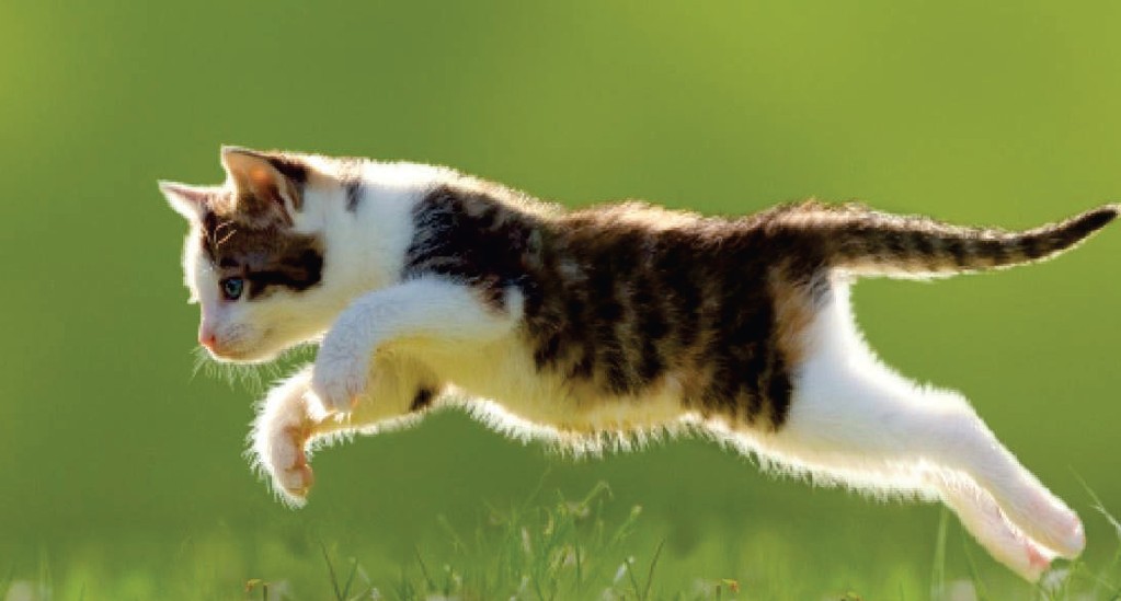
The dataset KYDerby25.txt contains information on each running of the Kentucky Derby since 1875. The speeds of the winning horses have been calculated (taking into account the change in track length in 1896).
Checkpoint 26.1.12. Winning Speed Scatterplot.

Produce a scatterplot of the winning speed vs. year. Describe the direction, form, and strength of the association in context.

Checkpoint 26.1.13. Track Condition Comparison.

Create a coded scatterplot using track condition. Discuss whether and how the association changes across the track conditions.
You have attempted of activities on this page.