Investigation 5.3: Near-Sightedness and Night Lights (cont.)

Section 24.4 Investigation 5.3: Near-Sightedness and Night Lights (cont.)

Exercises 24.4.1 The Study

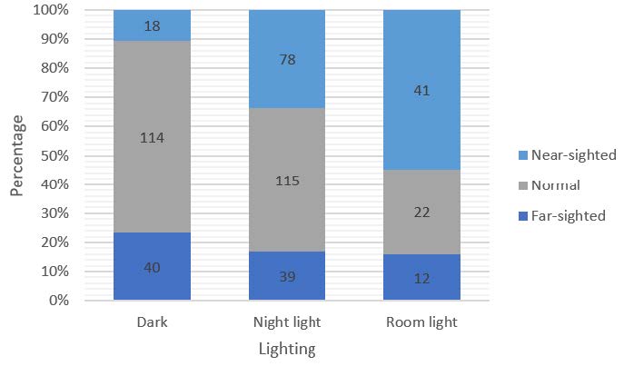
Recall Investigation 3.2, where we examined a simplified version of the Quinn, Shin, Maguire, and Stone (1999) study of childhood lighting exposure and eye refraction. Here we use three categories for each variable.

Eyes \ Lighting	Dark	Night light	Room light	Total
Far-sighted	40	39	12	91
Normal	114	115	22	251
Near-sighted	18	78	41	137
Total	172	232	75	479

Here we can view the data as one random sample cross-classified by lighting type and eye condition.

\(H_0\text{:}\) no association between lighting type and eye condition in the population.

\(H_a\text{:}\) there is an association.

This is a chi-squared test of association.

1. Simulation Plan.

Outline a simulation appropriate for this study design.

Solution.

We would need to randomly sample 479 individuals from a population with no association between the two variables. We could compute a chi-square statistic for each table and see how often we find a chi-square value like one in this study or more extreme.

When technical conditions are met, we generally use the chi-squared theoretical null model.

2. Expected Count Calculation.

Use the general formula to calculate how many of these 479 children you would expect to find in the Room light, far-sighted category.

Solution.

Room light and far sighted \(= 91 \times 75 / 479 \approx 14.25\text{.}\)

3. Check Conditions.

Do you think the chi-squared distribution is valid for this table? Explain how you are deciding.

Solution.

The smallest expected count is larger than 10, so the validity conditions are met.

4. Technology Output and Contributions.

Use technology to calculate the chi-squared statistic, verify the degrees of freedom, and find the p-value. Also display the chi-squared cell contributions; where do the largest differences lie?

Solution.

Applet output.

The darkness/myopia cell and the room light/myopia cell have the largest contributions. We observed a smaller rate of myopia in the darkness group and a higher rate of myopia in the room light group than we would have expected if there are no differences among the lighting populations.

5. Conclusions Paragraph.

Write a paragraph summarizing your conclusions, being sure to comment on significance, generalizability, and causation.

Solution.

See Summary Conclusion box.

Study Conclusions.

The segmented bar graph suggests near-sightedness increases with lighting level in this sample. A chi-squared test of association is appropriate because expected counts are sufficiently large. The p-value is extremely small, indicating strong evidence of association between lighting and eye condition in the population represented by this sample. The largest cell discrepancies are fewer near-sighted children than expected in the dark group and more than expected in the room-light group.

Because this is an observational study, a cause-and-effect conclusion is not warranted. Confounding variables (for example, parental vision and related household lighting choices) may explain part of the observed association. Generalization should also be cautious because children were not sampled as a simple random sample from all children.

Subsection 24.4.2 Practice Problem 5.3

The National Vital Statistics Reports provided data on gestation period for babies born in 2002. The following table classifies the births by the mother’s race and by the duration of the pregnancy:

Gestation \ Race	White (non-Hispanic)	Black (non-Hispanic)	Hispanic
Pre-term (under 37 weeks)	251,132	101,423	99,510
Full term (37-42 weeks)	1,885,189	435,923	692,314
Post-term (over 42 weeks)	149,898	36,896	64,997

Checkpoint 24.4.1. Chi-squared Test of Association.

Consider these observations as a random sample from the birth process in the U.S. and conduct a chi-squared test of whether these data suggest an association between race and length of gestation period. Report the hypotheses, validity of technical conditions, sketch of sampling distribution, test statistic, and p-value. [Provide the details of your calculations and/or relevant computer output.] Summarize your conclusion.

Checkpoint 24.4.2. Largest Cell Contributions.

Which 2-3 of the nine cells in the table contribute the most to the calculation of the \(\Chi^2\) test statistic? Is the observed count lower or higher than the expected count in those cells? Summarize what this reveals about the association between race and length of gestation period.

You have attempted of activities on this page.

Prev Top Next