Section2.4Turning Geometry and Radius of Curvature
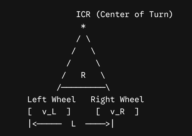
When a differential drive robot drives with constant unequal wheel speeds \((v_L \neq v_R)\text{,}\) it traces out a circular path around an Instantaneous Center of Rotation (ICR). The ICR is the single point in the plane that stays fixed while every other point on the robot, including both wheels, sweeps around it along its own circular arc at that instant.
An easy way to build intuition for the ICR is to picture the two wheels as if they were connected by a rigid rod (the axle) that is free to swing around some pivot point off to one side. If the two wheels move at the same speed, that pivot point is infinitely far away, and the "arc" they trace is really just a straight line. As the wheel speeds diverge, the pivot point moves closer to the robot, and the resulting circle gets tighter. Every differential drive turn, no matter how sharp or gentle, can be described by locating this single pivot point and computing the robot’s distance from it.
This formula is just \(v/\omega\) written two ways: the first form says "radius is how much forward distance you cover per unit of turning," which matches the everyday sense that a car going fast on a gentle curve has a large turn radius, while a robot spinning quickly with little forward motion has a tiny one. The second form expresses the same idea directly in terms of the two wheel speeds, which is often more convenient since those are the values a robot’s code actually has access to.
Real-World Example (Warehouse AMRs & Office Chairs): A warehouse Autonomous Mobile Robot barreling down a long, wide aisle prefers a large turn radius, sweeping into cross-aisles smoothly and quickly, much like a car merging onto a highway. But that same robot, when it needs to reorient in a tight, cluttered space between shelves, switches strategy entirely and spins in place (\(R = 0\)) to turn and face a new direction without needing any clearance to swing through. Choosing the right radius of curvature for the situation, wide and fast versus tight and stationary, is a real engineering decision every mobile robot’s motion planner has to make.
VEX AIM Robotics Example: All three turning scenarios above show up directly in VEX AIM competition strategy. A robot uses a point turn (\(R = 0\)) to quickly reorient toward a scoring goal without wasting time translating across the field. It uses a pivot turn (\(R = L/2\)) when one side of the robot is pinned against a field wall or another robot and only the free wheel can safely move. And it uses a smooth, finite-radius arc during autonomous routines when driving a curved path around field obstacles is faster than stopping, spinning, and re-accelerating in a straight line. Recognizing which scenario a given match situation calls for, and computing the wheel speeds to match, is exactly the skill this section builds.
Subsubsection2.4.4.1Exercise 2.4.1: Parsons Problem — Turning in a Perfect Circle of Radius \(R\)
Construct a Python script that calculates the required left and right wheel speeds \((v_L, v_R)\) to make a robot drive in a circle of radius \(R\) at a target linear speed \(v\text{.}\)
Arrange the blocks to form a complete function calculate_circular_wheel_speeds that computes the left and right wheel speeds needed to drive in a circle of radius \(R\) at linear speed \(v\text{.}\)