Section2.3Inverse Kinematics and Wheel Velocity Commands
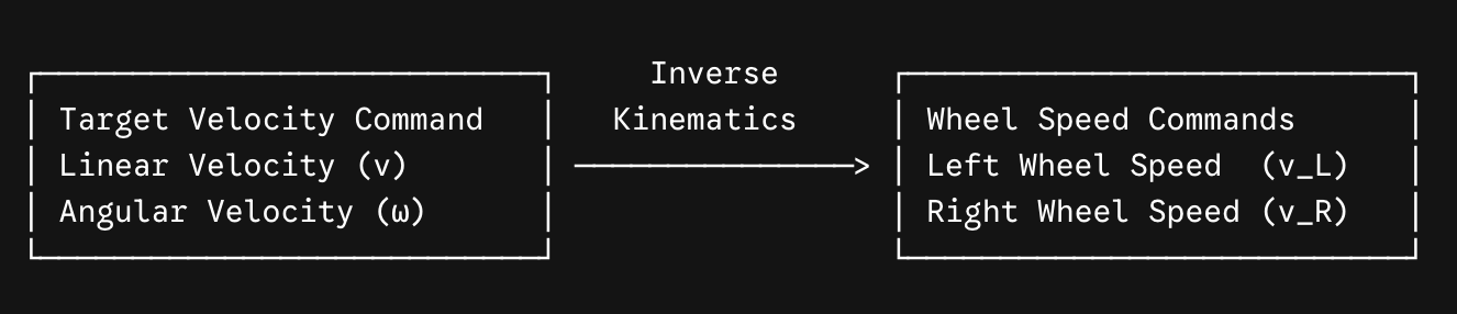
While forward kinematics calculates how the robot moves based on wheel speeds, inverse kinematics does the opposite: it takes a desired body motion velocity command \((v, \omega)\) and determines the required individual wheel surface velocities \((v_L, v_R)\text{.}\)
Given a target linear velocity \(v\) and angular velocity \(\omega\text{,}\) inverse kinematics produces the left wheel speed command \(v_L\) and the right wheel speed command \(v_R\) needed to achieve that motion.
This is the direction that actually matters for programming a robot’s autonomous behavior. A human, or an autonomous planning algorithm, thinks in terms of the robot’s overall motion—"drive forward at 0.5 m/s while turning slightly left"—not in terms of individual motor speeds. But the motors themselves have no concept of "the robot"; each one only understands "spin at this many radians per second." Inverse kinematics is the translation layer that sits between the high-level intent and the low-level motor commands, and it is running, quietly, every single time a robot changes speed or direction.
Notice this is exactly the forward kinematics equations solved backward: instead of starting from wheel speeds and finding \((v, \omega)\text{,}\) we start from the desired \((v, \omega)\) and add or subtract the same turning term \(\frac{\omega L}{2}\) to split it back into two wheel speeds. The final step—dividing by wheel radius \(r\)—exists because motors don’t control surface speed directly; they control how fast they spin, and a larger wheel covers more ground per rotation than a smaller one at the same spin rate.
Real-World Example (Autonomous Vehicle Steering): A self-driving car’s path planner decides on a high-level target: "follow this curve at 12 m/s with a turn rate of 0.3 rad/s." That plan means nothing to the vehicle’s actuators on its own. A lower-level controller performs an inverse-kinematics-style calculation to convert that single desired motion into the specific commands each wheel or steering actuator needs, the same fundamental problem solved here for a two-wheeled differential drive robot.
VEX AIM Robotics Example: During driver-controlled matches, a VEX AIM robot’s single-stick arcade drive code performs inverse kinematics roughly 50 times per second. The joystick’s forward/back axis is read as the desired linear velocity \(v\text{,}\) and its left/right axis is read as the desired angular velocity \(\omega\text{.}\) The controller code then applies these exact \(v_L\) and \(v_R\) formulas to compute how much power to send to the left and right drive motors—so every time a driver nudges the stick diagonally to "curve" the robot, they are triggering an inverse kinematics calculation without ever seeing the math.
Arrange the blocks to form a complete function compute_wheel_rpm that converts target body velocities \((v, \omega)\) into left and right wheel motor RPM values.
A robot with a track width \(L = 0.4\) m needs to execute a velocity command of linear speed \(v = 0.5\) m/s and angular speed \(\omega = 1.0\) rad/s. What are the required left and right wheel velocities \((v_L, v_R)\text{?}\)