Section 6.5 Model Evaluation: Classification, Confusion Matrices, and Regression Metrics

Once you train a machine learning model to detect objects or predict motor speeds, you need a way to measure how well it actually performs before deploying it to physical hardware. Evaluating a model relies on different metrics depending on whether the task is Classification (predicting discrete classes like "Obstacle" vs. "Free Space") or Regression (predicting continuous values like motor speed or object distance).

Subsection 6.5.1 Evaluating Classification: The Confusion Matrix & Accuracy

In classification, your model makes a discrete guess for every input. To see where it succeeds and where it makes dangerous mistakes, we organize its predictions into a Confusion Matrix.
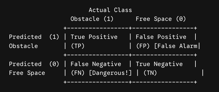
A Confusion Matrix is a grid that compares the ground-truth actual labels against the model’s predicted labels. For a binary obstacle-classification task, there are four possible outcomes:
Figure 6.5.1. Confusion matrix outcomes for binary classification.

Subsubsection 6.5.1.1 The Four Outcomes Explained

  1. True Positive (TP): The actual object is an Obstacle, and the model predicted Obstacle. This is correct.
  2. True Negative (TN): The actual space is Free Space, and the model predicted Free Space. This is correct.
  3. False Positive (FP): The space is actually Free Space, but the model predicted Obstacle. This false alarm causes the robot to stop unnecessarily.
  4. False Negative (FN): The object is actually an Obstacle, but the model predicted Free Space. This dangerous miss can cause the robot to crash into the obstacle.
Robotics Insight: In robotics, not all errors are equal. A False Positive (stopping for a shadow) causes a minor delay, but a False Negative (failing to detect a wall) can damage physical hardware.

Subsubsection 6.5.1.2 Classification Accuracy

Overall Accuracy measures the percentage of total predictions the model got correct:
\begin{equation*} \operatorname{Accuracy} = \frac{\mathrm{TP} + \mathrm{TN}}{\mathrm{TP} + \mathrm{TN} + \mathrm{FP} + \mathrm{FN}} \end{equation*}

Subsection 6.5.2 Evaluating Regression: MSE and \(R^2\) Score

When predicting continuous numerical valuesβ€”such as estimating the distance to a VEX game element in meters or calculating linear velocity \(v\)β€”we cannot use a confusion matrix. Instead, we measure how far the predicted numbers are from the actual values.
Actual Distance:     2.50 meters
Predicted Distance:  2.10 meters  --> Error = -0.40 meters

Subsubsection 6.5.2.1 Mean Squared Error (MSE)

Mean Squared Error (MSE) calculates the average of the squared differences between the actual values \(y\) and the predicted values \(\hat{y}\text{.}\)
\begin{equation*} \operatorname{MSE} = \frac{1}{n} \sum_{i=1}^{n} \left(y_i - \hat{y}_i\right)^2 \end{equation*}
Why square the errors?
  1. Squaring turns all errors into positive numbers so positive and negative errors do not cancel each other out.
  2. Squaring heavily penalizes large errors. Being off by \(2\text{ meters}\) is penalized four times as much as being off by \(1\text{ meter}\) because \(2^2 = 4\) while \(1^2 = 1\text{.}\) Lower MSE values indicate a better fit.

Subsubsection 6.5.2.2 R-Squared (\(R^2\)) Score (Coefficient of Determination)

While MSE describes squared error magnitude, \(R^2\) describes how well the model explains the variance in the dataset compared with a baseline that always predicts the dataset mean.
  • \(R^2 = 1.0\) (100%): Perfect predictions. Every prediction matches ground truth exactly.
  • \(R^2 = 0.0\) (0%): The model performs no better than always predicting the dataset’s average value.
  • \(R^2 < 0.0\) (negative): The model performs worse than always predicting the dataset average.

Reading Questions 6.5.3 Reading Questions

Check Your Understanding: 6.5

1. Exercise 6.5.1: Identifying a False Positive.

A VEX AI robot’s camera looks at an empty field tile and predicts "Red Ring Detected," causing the robot to lower its intake unnecessarily. Which confusion-matrix outcome does this represent?
  • True Positive (TP)
  • Incorrect. There was no ring in the ground truth.
  • True Negative (TN)
  • Incorrect. The model predicted a positive target rather than correctly identifying empty space.
  • False Positive (FP)
  • Correct. The ground truth is negative or empty, but the model incorrectly predicts a positive target.
  • False Negative (FN)
  • Incorrect. A false negative would miss a ring or obstacle that was actually present.

2. Exercise 6.5.2: Why MSE Squares Errors.

When evaluating a regression model that predicts continuous motor speed, why do we square prediction errors when calculating MSE?
  • Squaring converts continuous predictions into discrete classification labels.
  • Incorrect. MSE remains a regression metric for continuous values.
  • Squaring prevents negative and positive errors from canceling and penalizes larger errors more heavily.
  • Correct. Squaring makes every contribution nonnegative and gives large errors greater influence.
  • Squaring scales \(R^2\) values so they always remain above 100%.
  • Incorrect. \(R^2\) can be less than zero and is a separate metric.
  • Squaring allows Runestone to execute external C++ libraries.
  • Incorrect. The mathematical operation is unrelated to library support.

3. Exercise 6.5.3: ActiveCode Exercise β€” Pure Python Model Evaluation Metrics.

Runestone ActiveCode uses pure Python without external libraries such as scikit-learn or numpy, so this exercise implements the evaluation routines directly.
The two functions below calculate TP, TN, FP, and FN from binary labels and calculate the Mean Squared Error between actual and predicted distances.

4. Exercise 6.5.4: Parsons Problem β€” Assembling Confusion Matrix Logic.

Reorder the code blocks to construct the loop for counting True Positives and False Negatives in a binary classification evaluation script. Arrange the blocks to form a complete count_positives function that returns the TP and FN counts.
You have attempted of activities on this page.