Section 8.4 Maps Revisited: Skip Lists
One of the most versatile collections available in Java is the map. Maps, often referred to as dictionaries, store a collection of key-value pairs. The key, which must be unique, is assigned an association with a particular data value. Given a key, it is possible to ask the map for the corresponding associated data value. The abilities to put a key-value pair into the map and then look up a data value associated with a given key are the fundamental operations that all maps must provide.
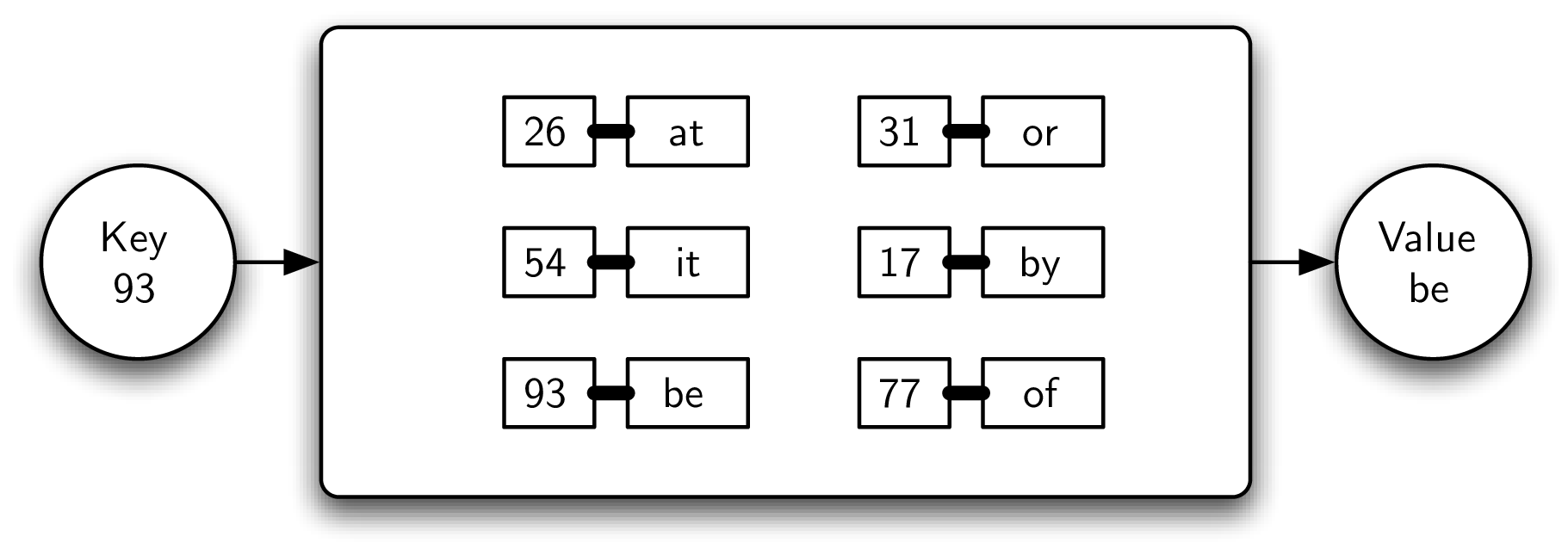
For example, Figure 8.4.1 shows a map containing key-value pairs. In this case, the keys are integers and the values are small, two-character words. From a logical perspective, there is no inherent order or organization within the pairs themselves. However, as the example shows, if a key (93) is provided to the map, the associated value (be) is returned.
Subsection 8.4.1 The Map Abstract Data Type
The map abstract data type is defined by the following structure and operations. The structure of a map, as described above, is a collection of key-value pairs where values can be accessed via their associated key. The map operations are given below:
-
Map()creates a new map that is empty. It needs no parameters and returns an empty map. -
put(key,value)adds a new key-value pair to the map. It needs the key and the associated value and returns nothing. Assume the key is not already in the map. -
get(key)searches for the key in the map and returns the associated value. It needs the key and returns a value.
It should be noted that there are a number of other possible operations that we could add to the map abstract data type. We will explore these in the exercises.
Subsection 8.4.2 Implementing a Map in Java
We have already seen a number of interesting ways to implement the map idea. In Chapter 5 we considered the hash table as a means of providing map behavior. Given a set of keys and a hash function, we could place the keys in a collection that allowed us to search and retrieve the associated data value. Our analysis showed that this technique could potentially yield an \(O(1)\) search. However, performance degraded due to issues such as table size, collisions, and collision resolution strategy.
In Chapter 6 we considered a binary search tree as a way to store such a collection. In this case the keys were placed in the tree such that searching could be done in \(O(\log n)\text{.}\) However, this was only true if the tree was balanced; that is, the left and the right subtrees were all of similar size. Unfortunately, depending on the order of insertion, the keys could end up being skewed to the right or to the left. In this case the search again degrades.
The problem we would like to address here is to come up with an implementation that has the advantages of an efficient search without the drawbacks described above. One such possibility is called a skip list. Figure 8.4.2 shows a possible skip list for the collection of key-value pairs shown in Figure 8.4.1 (the reason for saying “possible” will become apparent later). As you can see, a skip list is basically a two-dimensional linked list where the links all go forward (to the right) or down. The head of the list can be seen in the upper left corner. Note that this is the only entry point into the skip list structure.

Before moving on to the details of skip-list processing it will be useful to explain some vocabulary. Figure 8.4.3 shows that the majority of the skip list structure consists of a collection of data nodes, each of which holds a key and an associated value. In addition, there are two references from each data node. Figure 8.4.4 shows a detailed view of a single data node.
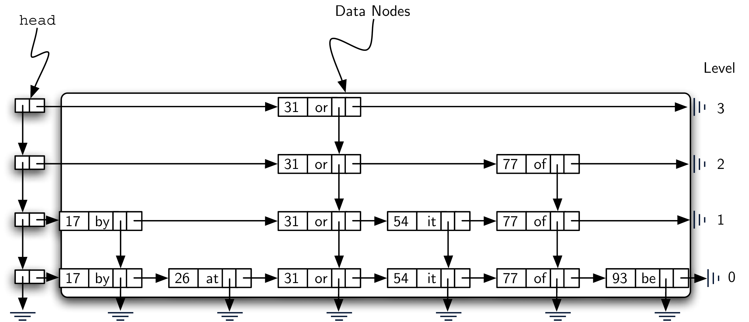

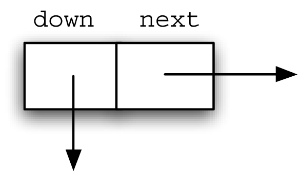
Figure 8.4.5 shows two different vertical columns. The leftmost column consists of a linked list of header nodes. Each header node holds two references called
down and next. The next reference refers to a linked list of data nodes. The down reference refers to the next lower header node. A detailed view of a header node can be seen in Figure 8.4.6.
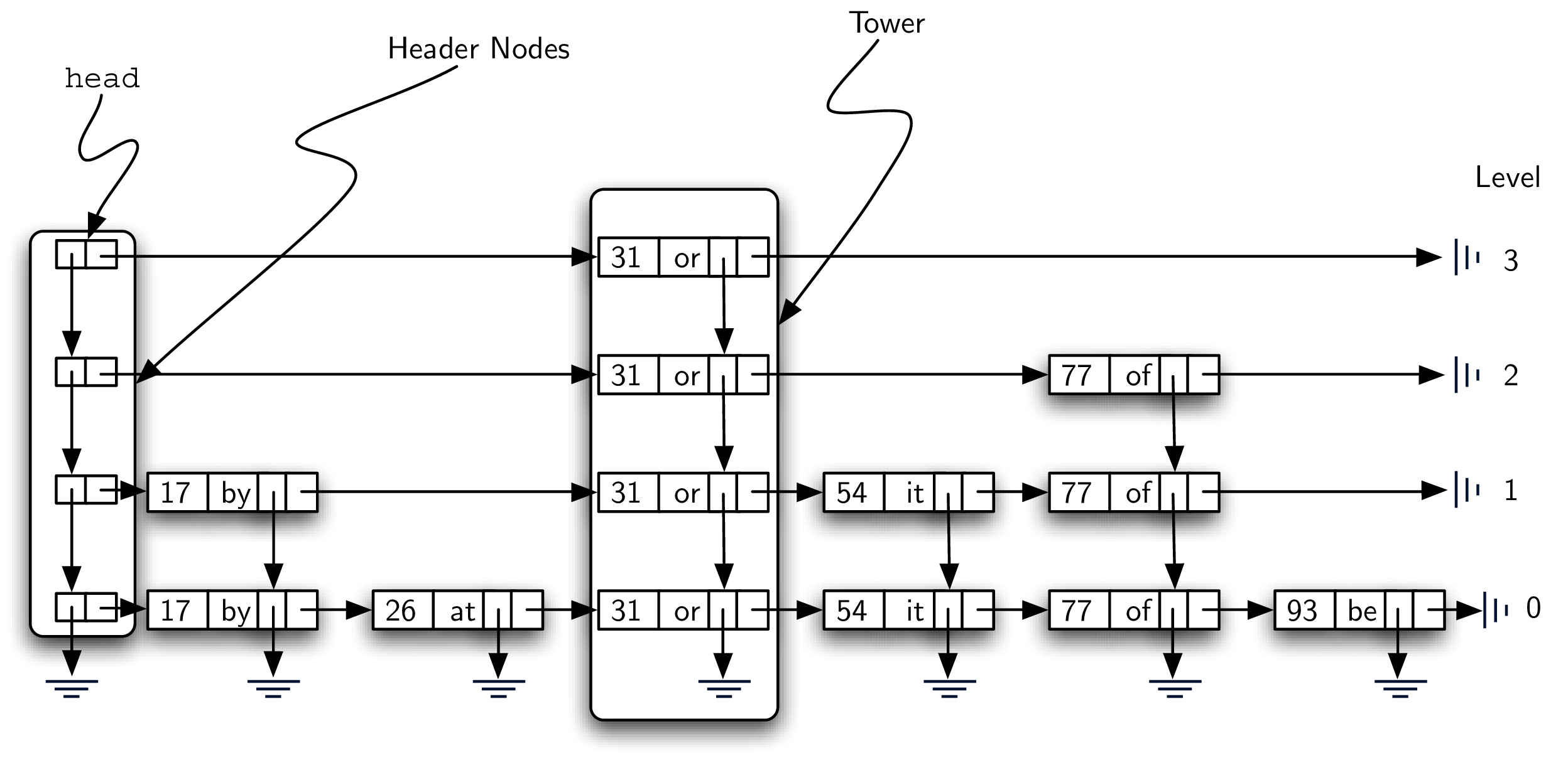
The columns of data nodes are known as towers. Towers are linked together by the
down reference in the data node. We can see that each tower corresponds to a particular key-value pair, and towers can have different heights. We will explain how the height of the tower is determined later when we consider how to add data to the skip list.
Finally, Figure 8.4.7 shows a horizontal collection of nodes. If you look closely, you will notice that each level is actually an ordered linked list of data nodes where the order is maintained by the key. Each linked list is given a name, commonly referred to as its level. Levels are named starting with 0 at the lowest row. Level 0 consists of the entire collection of nodes. Every key-value pair must be present in the level-0 linked list. However, as we move up to higher levels, we see that the number of nodes decreases. This is one of the important characteristics of a skip list and will lead to an efficient search. Again, it can be seen that the number of nodes at each level is directly related to the height of the towers.

While we could implement two different classes for
HeaderNode and DataNode, we will take the more convenient (or rather, hack-ish) option of creating only a “Skip List Node” SLNode. This will avoid needing to define DataNode as a subclass of HeaderNode with all the interesting casts and compile-time checking that Java would enforce. When we create a SLNode as a header, its key and value fields will both be null.
This class can be constructed in the same fashion as for simple linked lists. An
SLNode node consists of two references, next and down, both of which are initialized to null in the constructor (see Listing 8.4.8), and a key and value field, which are null. We also provide a constructor that lets you initialize the key and value:
SLNode Classclass SLNode<K extends Comparable<K>, V> {
private SLNode<K, V> next;
private SLNode<K, V> down;
private K key;
private V value;
public SLNode() {
this.next = null;
this.down = null;
this.key = null;
this.value = null;
}
public SLNode(K key, V value) {
this.next = null;
this.down = null;
this.key = key;
this.value = value;
}
public SLNode<K, V> getNext() {
return this.next;
}
public void setNext(SLNode<K, V> next) {
this.next = next;
}
public SLNode<K, V> getDown() {
return this.down;
}
public void setDown(SLNode<K, V> down) {
this.down = down;
}
public K getKey() {
return this.key;
}
public V getValue() {
return this.value;
}
}
The constructor for the entire skip list is shown in Listing 8.4.9, as well as the getters and setters for the
head property. When a skip list is created, there are no data and therefore no header nodes. The head of the skip list is set to null. As key-value pairs are added to the structure, the list head refers to the first header node which in turn provides access to a linked list of data nodes as well as access to lower levels.
class SkipList<K extends Comparable<K>, V> {
    private SLNode<K, V> head;

    public SkipList() {
        this.head = null;
    }

    public SLNode<K, V> getHead() {
        return this.head;
    }

    public void setHead(SLNode<K, V> head) {
        this.head = head;
    }
Subsubsection 8.4.2.1 Searching a Skip List
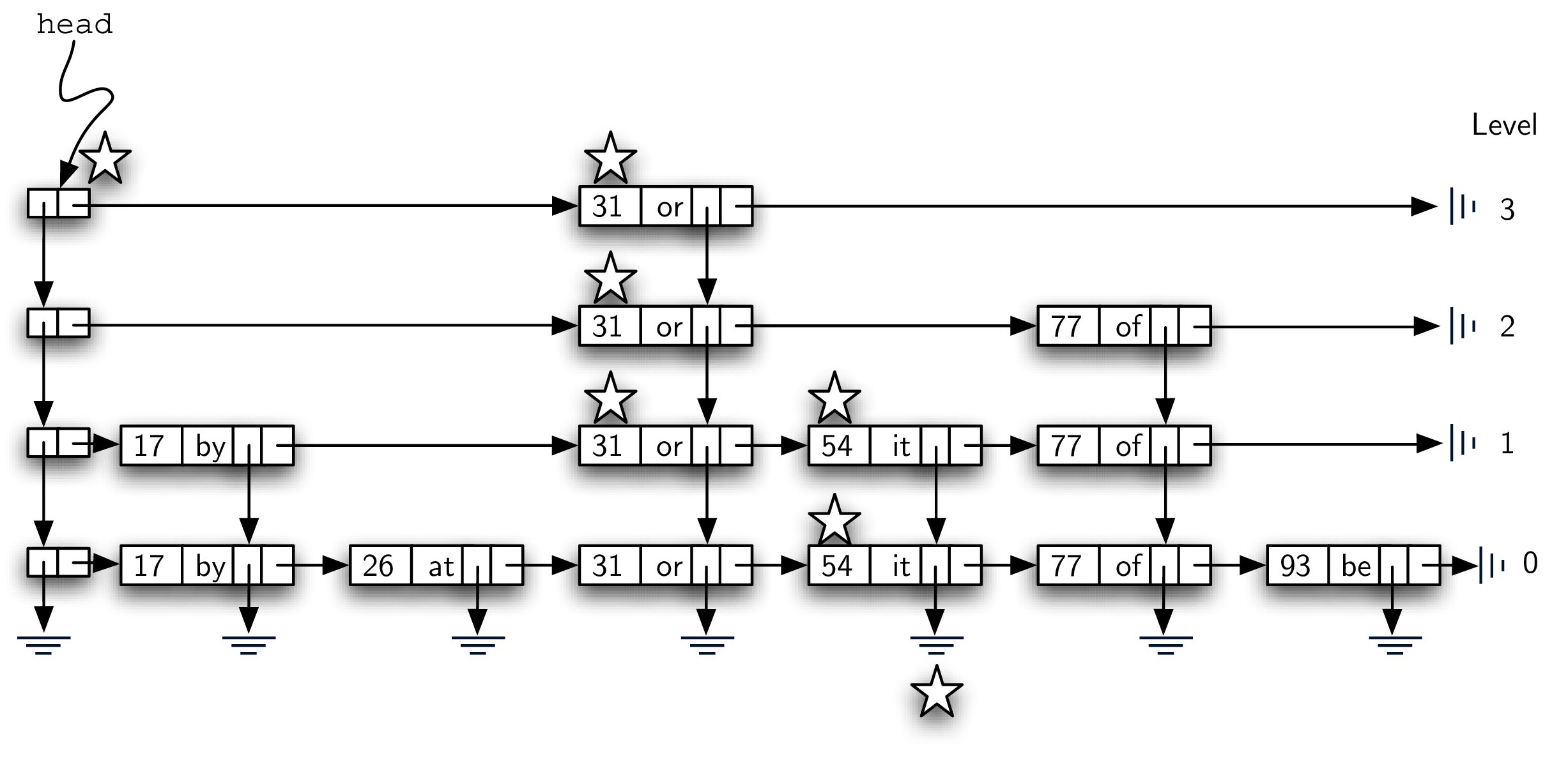
The search operation for a skip list will require a key. It will find a data node containing that key and return the corresponding value that is stored in the node. Figure 8.4.10 shows the search process as it proceeds through the skip list looking for the key 77. The nodes marked by stars represent those that are considered during the search process.

As we search for 77, we begin at the head of the skip list. The first header node refers to the data node holding 31. Since 31 is less than 77, we move forward. Now since there is no next data node from 31 at that level (level 3), we must drop down to level 2. This time, when we look to the right, we see a data node with the key 77. Our search is successful and the word of is returned. It is important to note that our first comparison, data node 31, allowed us to skip over 17 and 26. Likewise, from 31 we were able to go directly to 77, bypassing 54.
The following code block shows the Java implementation of the
search method. The search starts at the head of the list and searches through nodes until either the key is found or there are no more nodes to check. The basic idea is to start at the header node of the highest level and begin to look to the right. If no data node is present, the search continues on the next lower level (lines 4-5). On the other hand, if a data node exists, we compare the keys. If there is a match, we have found a data node with the key we are looking for and we can return its value (lines 7-8).
public V search(K key) {
    SLNode<K, V> current = this.head;
    while (current != null) {
        if (current.getNext() == null) {
            current = current.getDown();
        } else {
            K testKey = current.getNext().getKey();
            if (testKey.equals(key)) {
                return current.getNext().getValue();
            }
            if (key.compareTo(testKey) < 0) {
                current = current.getDown();
            } else {
                current = current.getNext();
            }
        }
    }
    return null;
}
Since each level is an ordered linked list, a key mismatch provides us with very useful information. If the key we are looking for is less than the key contained in the data node (line 11), we know that no other data node on that level can contain our key since everything to the right has to be greater. In that case, we drop down one level in that tower (line 12). If no such level exists (we drop to
null), we have discovered that the key is not present in our skip list. We break out of the loop and return null. On the other hand, as long as there are data nodes on the current level with key values less than the key we are looking for, we continue moving to the next node (line 14).
Once we enter a lower level, we repeat the process of checking to see if there is a next node. Each level lower in the skip list has the potential to provide additional data nodes. If the key is present, it will have to be discovered no later than level 0 since level 0 is the complete ordered linked list. Our hope is that we will find it sooner.
Subsubsection 8.4.2.2 Adding Key-Value Pairs to a Skip List
If we are given a skip list, the
search method is fairly easy to implement. Our task here is to understand how the skip list structure was built in the first place and how it is possible that the same set of keys, added in the same order, can give us different skip lists.
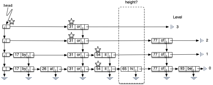
Adding a new key-value pair to the skip list is essentially a two-step process. First, we search the skip list looking for the position where the key should have been. Remember that we are assuming the key is not already present. Figure 8.4.12 shows this process as we look to add the key 65 (data value “hi”) to the collection. We have used the stars once again to show the path of the search process as it proceeds through the skip list.
As we proceed using the same search strategy as in the previous section, we find that 65 is greater than 31. Since there are no more nodes on level 3, we drop to level 2. Here we find 77, which is greater than 65. Again, we drop, this time to level 1. Now the next node is 54, which is less than 65. Continuing to the right, we hit 77, which again causes us to drop down until eventually we hit the
null at the base of the tower.
The second step in the process is to create a new data node and add it to the level 0 linked list (Figure 8.4.13). However, if we stop at that point, the best we will ever have is a single linked list of key-value pairs. We also need to build a tower for the new entry, and this is where the skip list gets very interesting. How high should the tower be? The height of the tower for the new entry will not be predetermined but instead will be completely probabilistic. In essence, we will flip a coin to decide whether to add another level to the tower. Each time the coin comes up heads, we will add one more level to the current tower.
We will use the
Math.random() method to simulate coin flip, with 0 as tails and 1 as heads.
Listing 8.4.14 shows the
insert method. Lines 2–4 define some variables we will need multiple times throughout the code. You will note immediately in line 6 that we need to check to see if this is the first node being added to the skip list. This is the same question we asked for simple linked lists. If we are adding to the head of the list, a new header node as well as data node must be created. The iteration in lines 11–19 continues as long as the randrange function returns a 1 (the coin toss returns heads). Each time a new level is added to the tower, a new data node and a new header node are created (lines 12–13).
In the case of a non-empty skip list (line 20), we need to search for the insert position as described above. Since we have no way of knowing how many data nodes will be added to the tower, we need to save the insert points for every level that we enter as part of the search process. These insert points will be processed in reverse order, so a stack will work nicely to allow us to back up through the linked lists inserting tower data nodes as necessary. The stars in Figure 8.4.13 show the insert points that would be stacked in the example. These points represent only those places where we dropped down during the search.
Starting at line 43, we flip our coin to determine the number of levels for the tower. This time we pop the insert stack (line 53) to get the next higher insertion point as the tower grows. Only after the stack becomes empty will we need to return to creating new header nodes. We leave the remaining details of the implementation for you to trace.
public void insert(K key, V value) {
    SLNode<K, V> temp;
    SLNode<K, V> top;
    SLNode<K, V> newHead;

    if (head == null) {
        this.head = new SLNode<K, V>();
        temp = new SLNode<K, V>(key, value);
        this.head.setNext(temp);
        top = temp;
        while ((int) (Math.random() * 2) == 1) {
            newHead = new SLNode<K, V>();
            temp = new SLNode<K, V>(key, value);
            temp.setDown(top);
            newHead.setNext(temp);
            newHead.setDown(this.head);
            this.head = newHead;
            top = temp;
        }
    } else {
        Stack<SLNode<K, V>> tower = new Stack<>();
        SLNode<K, V> current = this.head;
        while (current != null) {
            if (current.getNext() == null) {
                tower.push(current);
                current = current.getDown();
            } else {
                if (current.getNext().getKey().compareTo(key) > 0) {
                    tower.push(current);
                    current = current.getDown();
                } else {
                    current = current.getNext();
                }
            }
        }

        SLNode<K, V> lowestLevel = tower.pop();
        temp = new SLNode<>(key, value);
        temp.setNext(lowestLevel.getNext());
        lowestLevel.setNext(temp);
        top = temp;

        while ((int) (Math.random() * 2) == 1) {
            if (tower.isEmpty()) {
                newHead = new SLNode<K, V>();
                temp = new SLNode<K, V>(key, value);
                temp.setDown(top);
                newHead.setNext(temp);
                newHead.setDown(this.head);
                this.setHead(newHead);
                top = temp;
            } else {
                SLNode<K, V> nextLevel = tower.pop();
                temp = new SLNode<K, V>(key, value);
                temp.setDown(top);
                temp.setNext(nextLevel.getNext());
                nextLevel.setNext(temp);
                top = temp;
            }
        }
    }
}
We should make one final note about the structure of the skip list. We had mentioned earlier that there are many possible skip lists for a set of keys, even if they are inserted in the same order. Now we see why. Depending on the random nature of the coin flip, the height of the towers for any particular key is bound to change each time we build the skip list.
Subsubsection 8.4.2.3 Building the Map
Now that we have implemented the skip list behavior allowing us to add data to the list and search for data that is present, we are in a position to finally implement the map abstract data type. As we discussed above, maps must provide two operations,
put and get. Listing 8.4.15 shows that these operations can be implemented by constructing an internal skip list collection and using the insert and search operations shown in the previous two sections.
Map Classclass Map<K extends Comparable<K>, V> {
private SkipList<K, V> collection;
public Map() {
this.collection = new SkipList<K, V>();
}
public void put(K key, V value) {
this.collection.insert(key, value);
}
public V get(K key) {
return this.collection.search(key);
}
public SkipList<K, V> getCollection() {
return this.collection;
}
}
Here is a diagram of the result of inserting the keys and values shown in Figure 8.4.1:
| --> 17/by --> 26/at --------------------------------> 93/be
| --> 17/by --> 26/at --> 31/or ----------------------> 93/be
| --> 17/by --> 26/at --> 31/or --> 54/it --> 77/of --> 93/be
Subsubsection 8.4.2.4 Analysis of a Skip List
If we had simply stored the key-value pairs in an ordered linked list, we know that the search method would be \(O(n)\text{.}\) Can we expect better performance from the skip list? Recall that the skip list is a probabilistic data structure. This means that the analysis will be dependent upon the probability of some event, in this case, the flip of a coin. Although a rigorous analysis of this structure is beyond the scope of this text, we can make a strong informal argument.
Assume that we are building a skip list for \(n\) keys. We know that each tower starts off with a height of 1. As we add data nodes to the tower, assuming the probability of getting heads is \(\frac{1}{2}\text{,}\) we can say that \(\frac{n}{2}\) of the keys have towers of height 2. As we flip the coin again, \(\frac{n}{4}\) of the keys have a tower of height 3. This corresponds to the probability of flipping two heads in a row. Continuing this argument shows \(\frac{n}{8}\) keys have a tower of height 4 and so on. This means that we expect the height of the tallest tower to be \(\log_{2}(n) + 1\text{.}\) Using our Big-O notation, we would say that the height of the skip list is \(O(\log (n))\text{.}\)
To analyze the
search method, recall that there are two scans that need to be considered as we look for a given key. The first is the down direction. The previous result suggests that in the worst case we will expect to consider \(O(\log (n))\) levels to find a key. In addition, we need to include the number of forward links that need to be scanned on each level. We drop down a level when one of two events occurs. Either we find a data node with a key that is greater than the key we are looking for or we find the end of a level. If we are currently looking at some data node, the probability that one of those two events will happen in the next link is \(\frac{1}{2}\text{.}\) This means that after looking at two links, we would expect to drop to the next lower level (we expect to get heads after two coin flips). In any case, the number of nodes that we need to look at on any given level is constant. The entire result then becomes \(O(\log (n))\text{.}\) Since inserting a new node is dominated by searching for its location, the insert operation will also have \(O(\log(n))\) performance.
You have attempted of activities on this page.
