t Probability Table

Section B.3 \(t\) Probability Table

A \(t\)-probability table may be used to find tail areas of a t-distribution using a T-score, or vice-versa. Such a table lists T-scores and the corresponding percentiles. A partial t-table is shown in Table B.3.1, and the complete table starts further below. Each row in the t-table represents a t-distribution with different degrees of freedom. The columns correspond to tail probabilities. For instance, if we know we are working with the t-distribution with \(df = 18\text{,}\) we can examine row 18, which is highlighted in Table B.3.1. If we want the value in this row that identifies the T-score (cutoff) for an upper tail of 10%, we can look in the column where one tail is 0.100. This cutoff is 1.33. If we had wanted the cutoff for the lower 10%, we would use -1.33. Just like the normal distribution, all t-distributions are symmetric.

Table B.3.1. An abbreviated look at the t-table. Each row represents a different t-distribution. The columns describe the cutoffs for specific tail areas. The row with \(df = 18\) has been emphasized.

one tail		0.100	0.050	0.025	0.010	0.005
two tails		0.200	0.100	0.050	0.020	0.010
df	1	3.08	6.31	12.71	31.82	63.66
	2	1.89	2.92	4.30	6.96	9.92
	3	1.64	2.35	3.18	4.54	5.84
	\(\vdots\)	\(\vdots\)	\(\vdots\)	\(\vdots\)	\(\vdots\)
	17	1.33	1.74	2.11	2.57	2.90
	18	1.33	1.73	2.10	2.55	2.88
	19	1.33	1.73	2.09	2.54	2.86
	20	1.33	1.72	2.09	2.53	2.85
	\(\vdots\)	\(\vdots\)	\(\vdots\)	\(\vdots\)	\(\vdots\)
	400	1.28	1.65	1.97	2.34	2.59
	500	1.28	1.65	1.96	2.33	2.59
	\(\infty\)	1.28	1.64	1.96	2.33	2.58

Example B.3.2.

What proportion of the t-distribution with 18 degrees of freedom falls below -2.10?

Solution.

Just like a normal probability problem, we first draw the picture and shade the area below -2.10:

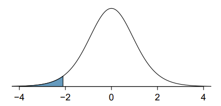
To find this area, we first identify the appropriate row: df = 18. Then we identify the column containing the absolute value of -2.10; it is the third column. Because we are looking for just one tail, we examine the top line of the table, which shows that a one tail area for a value in the third row corresponds to 0.025. That is, 2.5% of the distribution falls below -2.10.

In the next example we encounter a case where the exact T-score is not listed in the table.

Example B.3.3.

A t-distribution with 20 degrees of freedom is shown in the left panel of Figure B.3.4. Estimate the proportion of the distribution falling above 1.65.

Solution.

We identify the row in the t-table using the degrees of freedom: \(df = 20\text{.}\) Then we look for 1.65; it is not listed. It falls between the first and second columns. Since these values bound 1.65, their tail areas will bound the tail area corresponding to 1.65. We identify the one tail area of the first and second columns, 0.050 and 0.10, and we conclude that between 5% and 10% of the distribution is more than 1.65 standard deviations above the mean. If we like, we can identify the precise area using statistical software: 0.0573.

Figure B.3.4. Left: The t-distribution with 20 degrees of freedom, with the area above 1.65 shaded. Right: The t-distribution with 475 degrees of freedom, with the area further than 2 units from 0 shaded.

Example B.3.5.

A t-distribution with 475 degrees of freedom is shown in the right panel of Figure B.3.4. Estimate the proportion of the distribution falling more than 2 units from the mean (above or below).

Solution.

As before, first identify the appropriate row: \(df = 475\text{.}\) This row does not exist! When this happens, we use the next smaller row, which in this case is \(df = 400\text{.}\) Next, find the columns that capture 2.00; because \(1.97 \lt 3 \lt 2.34\text{,}\) we use the third and fourth columns. Finally, we find bounds for the tail areas by looking at the two tail values: 0.02 and 0.05. We use the two tail values because we are looking for two symmetric tails in the t-distribution.

Guided Practice B.3.6.

What proportion of the t-distribution with 19 degrees of freedom falls above -1.79 units?

We find the shaded area above -1.79 (we leave the picture to you). The small left tail is between 0.025 and 0.05, so the larger upper region must have an area between 0.95 and 0.975.

Example B.3.7.

Find the value of \(t^{*}_{18}\) using the t-table, where \(t^{*}_{18}\) is the cutoff for the t-distribution with 18 degrees of freedom where 95% of the distribution lies between \(-t^{*}_{18}\) and \(+t^{*}_{18}\text{.}\)

Solution.

For a 95% confidence interval, we want to find the cutoff \(t^{*}_{18}\) such that 95% of the t-distribution is between \(-t^{*}_{18}\) and \(+t^{*}_{18}\text{;}\) this is the same as where the two tails have a total area of 0.05. We look at the full t-table below, find the column with area totaling 0.05 in the two tails (third column), and then the row with 18 degrees of freedom: \(+t^{*}_{18}=2.10\text{.}\)

Table B.3.9.


one tail		0.100	0.050	0.025	0.010	0.005
two tail		0.200	0.100	0.050	0.020	0.010
df	1	3.08	6.31	12.71	31.82	63.66
	2	1.89	2.92	4.30	6.96	9.92
	3	1.64	2.35	3.18	4.54	5.84
	4	1.53	2.13	2.78	3.75	4.60
	5	1.48	2.02	2.57	3.36	4.03
	6	1.44	1.94	2.45	3.14	3.71
	7	1.41	1.89	2.36	3.00	3.50
	8	1.40	1.86	2.31	2.90	3.36
	9	1.38	1.83	2.26	2.82	3.25
	10	1.37	1.81	2.23	2.76	3.17
	11	1.36	1.80	2.20	2.72	3.11
	12	1.36	1.78	2.18	2.68	3.05
	13	1.35	1.77	2.16	2.65	3.01
	14	1.35	1.76	2.14	2.62	2.98
	15	1.34	1.75	2.13	2.60	2.95
	16	1.34	1.75	2.12	2.58	2.92
	17	1.33	1.74	2.11	2.57	2.90
	18	1.33	1.73	2.10	2.55	2.88
	19	1.33	1.73	2.09	2.54	2.86
	20	1.33	1.72	2.09	2.53	2.85
	21	1.32	1.72	2.08	2.52	2.83
	22	1.32	1.72	2.07	2.51	2.82
	23	1.32	1.71	2.07	2.50	2.81
	24	1.32	1.71	2.06	2.49	2.80
	25	1.32	1.71	2.06	2.49	2.79
	26	1.31	1.71	2.06	2.48	2.78
	27	1.31	1.70	2.05	2.47	2.77
	28	1.31	1.70	2.05	2.47	2.76
	29	1.31	1.70	2.05	2.46	2.76
	30	1.31	1.70	2.04	2.46	2.75

Table B.3.11.


one tail		0.100	0.050	0.025	0.010	0.005
two tail		0.200	0.100	0.050	0.020	0.010
df	31	1.31	1.70	2.04	2.45	2.74
	32	1.31	1.69	2.04	2.45	2.74
	33	1.31	1.69	2.03	2.44	2.73
	34	1.31	1.69	2.03	2.44	2.73
	35	1.31	1.69	2.03	2.44	2.72
	36	1.31	1.69	2.03	2.43	2.72
	37	1.30	1.69	2.03	2.43	2.72
	38	1.30	1.69	2.02	2.43	2.71
	39	1.30	1.68	2.02	2.43	2.71
	40	1.30	1.68	2.02	2.42	2.70
	41	1.30	1.68	2.02	2.42	2.70
	42	1.30	1.68	2.02	2.42	2.70
	43	1.30	1.68	2.02	2.42	2.70
	44	1.30	1.68	2.02	2.41	2.69
	45	1.30	1.68	2.01	2.41	2.69
	46	1.30	1.68	2.01	2.41	2.69
	47	1.30	1.68	2.01	2.41	2.68
	48	1.30	1.68	2.01	2.41	2.68
	49	1.30	1.68	2.01	2.40	2.68
	50	1.30	1.68	2.01	2.40	2.68
	60	1.30	1.67	2.00	2.39	2.66
	70	1.29	1.67	1.99	2.38	2.65
	80	1.29	1.66	1.99	2.37	2.64
	90	1.29	1.66	1.99	2.37	2.63
	100	1.29	1.66	1.98	2.36	2.63
	150	1.29	1.66	1.98	2.35	2.61
	200	1.29	1.65	1.97	2.35	2.60
	300	1.28	1.65	1.97	2.34	2.59
	400	1.28	1.65	1.97	2.34	2.59
	500	1.28	1.65	1.96	2.33	2.59
	\(\infty\)	1.28	1.65	1.96	2.33	2.58

You have attempted of activities on this page.

Prev Top Next