Normal distribution

Section 2.3 Normal distribution

What proportion of adults have systolic blood pressure above 140? What is the probability of getting more than 250 heads in 400 tosses of a fair coin? If the average weight of a piece of carry-on luggage is 11 pounds, what is the probability that 200 random carry on pieces will weigh more than 2500 pounds? If 55% of a population supports a certain candidate, what is the probability that she will have less than 50% support in a random sample of size 200?

There is one distribution that can help us answer all of these questions. Can you guess what it is? That’s right — it’s the normal distribution.

Objectives: Learning objectives

Use Z-scores and the standard normal model to approximate a distribution where appropriate.
Find probabilities and percentiles using the normal approximation.
Find the value that corresponds to a given percentile when the distribution is approximately normal.

Subsection 2.3.1 Normal distribution model

Among all the distributions we see in practice, one is overwhelmingly the most common. The symmetric, unimodal, bell curve is ubiquitous throughout statistics. Indeed it is so common, that people often know it as the normal curve or normal distribution.

It is also introduced as the Gaussian distribution after Frederic Gauss, the first person to formalize its mathematical expression.

A normal curve is shown in Figure 2.3.1.

The normal distribution always describes a symmetric, unimodal, bell-shaped curve. However, these curves can look different depending on the details of the model. Specifically, the normal distribution model can be adjusted using two parameters: mean and standard deviation. As you can probably guess, changing the mean shifts the bell curve to the left or right, while changing the standard deviation stretches or constricts the curve. Figure 2.3.2 shows the normal distribution with mean \(0\) and standard deviation \(1\) in the left panel and the normal distributions with mean \(19\) and standard deviation \(4\) in the right panel. Figure 2.3.3 shows these distributions on the same axis.

Figure 2.3.2. Both curves represent the normal distribution. However, they differ in their center and spread.

Figure 2.3.3. The normal distributions shown in Figure 2.3.2 but plotted together and on the same scale.

Because the mean and standard deviation describe a normal distribution exactly, they are called the distribution’s parameters. The normal distribution with mean \(\mu=0\) and standard deviation \(\sigma = 1\) is called the standard normal distribution..

Normal distribution facts.

Many variables are nearly normal, but none are exactly normal. The normal distribution, while never perfect, provides very close approximations for a variety of scenarios. We will use it to model data as well as probability distributions.

Subsection 2.3.2 Using the normal distribution to approximate empirical distributions

We often want to put data onto a standardized scale, which can make comparisons more reasonable.

Example 2.3.4.

Table 2.3.5 shows the mean and standard deviation for total scores on the SAT and ACT. The distribution of SAT and ACT scores are both nearly normal. Suppose Ann scored 1300 on her SAT and Tom scored 24 on his ACT. Who performed better?

Solution.

As we saw in Subsection 2.2.3, we can use Z-scores to compare observations from diferent distributions. Using Ann’s SAT score, 1300, along with the SAT mean and SD, we can find Ann’s Z-scores.

\(Z_{\text{Ann}} = \frac{x_{\text{Ann}}-\mu_{\text{SAT}}}{\sigma_{\text{SAT}}} = \frac{1300-1100}{200} = 1\)

Similarly, using Tom’s ACT score, 24, along with the ACT mean and SD we can find his Z-scores.

\(Z_{\text{Tom}} = \frac{x_{\text{Tom}}-\mu_{\text{ACT}}}{\sigma_{\text{ACT}}} = \frac{24-21}{6} = 0.5\)

Because Ann’s score was 1 standard deviation above the mean, while Tom’s score was 0.5 standard deviations above the mean, we can say that Ann did better than Tom.

Table 2.3.5. Mean and standard deviation for the SAT and ACT.


	SAT	ACT
Mean	1100	21
SD	200	6

Assuming that both the that both the SAT and ACT distributions are nearly normally distributed, what percent of test takers scored lower than Ann? What percent scored lower than Tom? To answer these question exactly, we would need all of the data. However, if we use the information that SAT and ACT distributions are nearly normal, we can estimate these percents. Figure 2.3.6 shows these distributions modeled with a normal curve. If we can find the percent of the normal curve that is to the left of Ann’s score, we could use that percent as our estimate of the percent of the data points that are smaller than Ann’s score. We call this process normal approximation. The steps are:

First verify that the distribution can be reasonably modeled with a normal distribution.
Convert value or values of interest to Z-scores.
Find the relevant area/percent under the standard normal curve.

We use the area/percent that we find from the normal curve as our estimate of the desired percent.

Figure 2.3.6. Ann’s and Tom’s scores shown with the distributions of SAT and ACT scores.

Subsection 2.3.3 Finding areas under the normal curve

It’s very useful in statistics to be able to identify areas of distributions, especially tail areas. For instance, what percent of people have an SAT score below Ann’s score of 1300? This is the same as Ann’s percentile. We previously determined that a score of 1300 corresponds to a Z-score of 1 and that SAT scores are approximately normally distributed. We can visualize such a tail area by sketching a normal curve and shading everything below \(Z = 1\) as shown in Table 2.3.5.

Figure 2.3.7. The area to the left of the Z-score represents the percentile of the observation

There are many techniques for finding this area, and we’ll discuss three of the options.

The most common approach in practice is to use statistical software. For example, in the program R, we could find the area shown in Figure 2.3.7 using the following command, which takes in the Z-score of 1 and returns the lower tail area:
```
> pnorm(1)
[1] 0.8413447
```
Using the online Desmos calculator, we could do: normaldist( ), check the “Find Cumulative Probability (CDF)” box and set Max to 1.

According to these calculation, the area shaded that is below \(Z = 1\) is 0.841, so we estimate that 84.1% of SAT test takers score below 1300 and that Ann is at the 84th percentile. There are many other software options, such as Pythn or SAS; even spreadsheet programs such as Excel and Google Sheets support these calculations.
A common strategy in classrooms is to use a graphing calculator, such as a TI or Casio calculator. Instructions for finding areas of a normal distribution using these calculators are provided in Subsection 2.3.7.
The last option for finding tail areas is to use what’s called a probability table; these are occasionally used in classrooms but rarely in practice. Section B.2 contains such a table and a guide for how to use it.

We will solve normal distribution problems in this section by always first finding the Z-score. The reason is that we will encounter close parallels called test statistics beginning in Chapter 5; these are, in many instances, an equivalent of a Z-score.

Readers may find it helpful to familiarize themselves with one of the options above before continuing on to the applications that follow.

Subsection 2.3.4 Normal probability examples

Combined SAT scores are approximated well by a normal model with mean 1100 and standard deviation 200.

Example 2.3.8.

What is the probability that a randomly selected SAT taker scores at least 1190 on the SAT?

Solution.

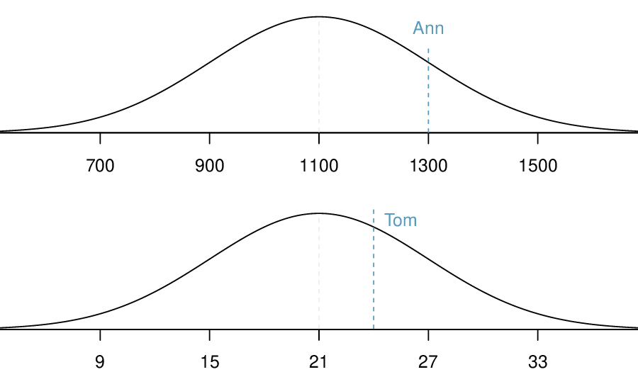
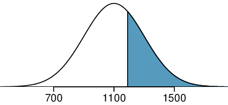
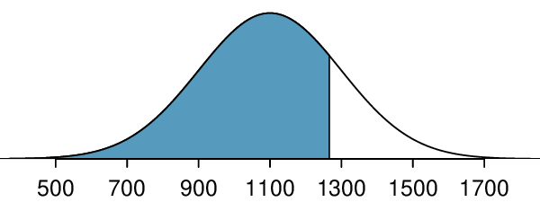
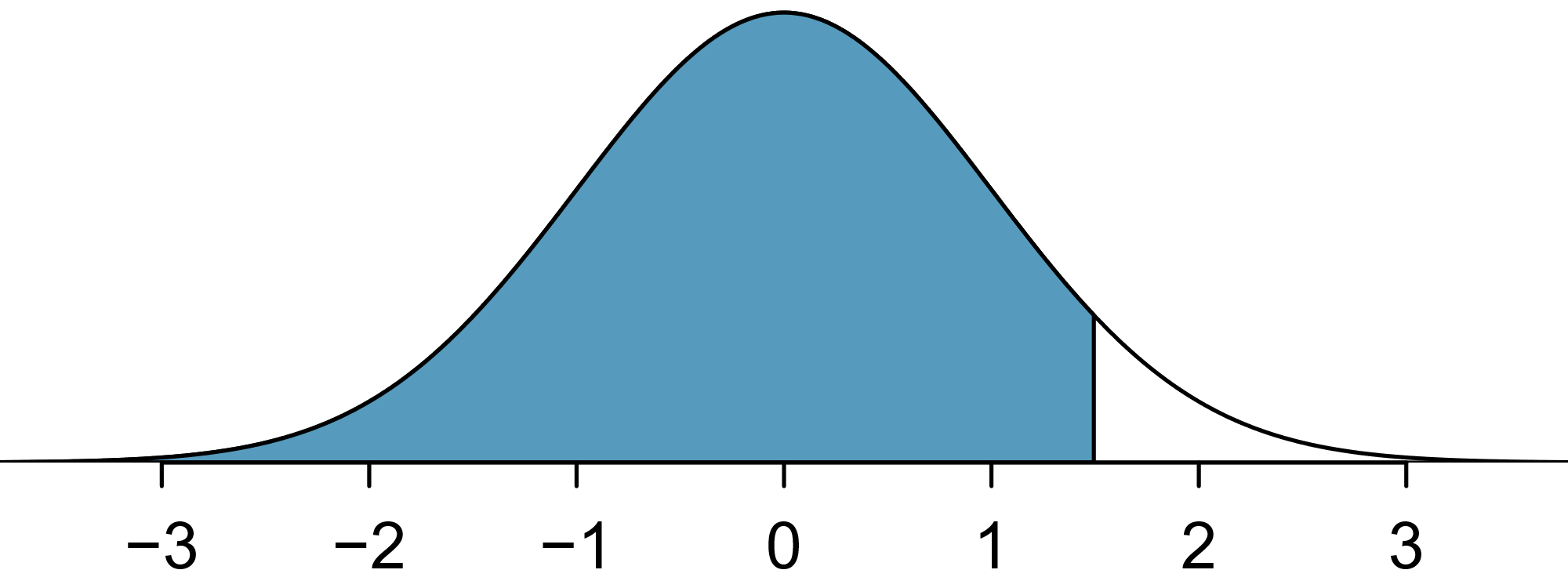
The probability that a randomly selected SAT taker scores at least 1190 on the SAT is equivalent to the proportion of all SAT takers that score at least 1190 on the SAT. First, always draw and label a picture of the normal distribution. (Drawings need not be exact to be useful.) We are interested in the probability that a randomly selected score will be above 1190, so we shade this upper tail:

The picture shows the mean and the values at 2 standard deviations above and below the mean. The simplest way to find the shaded area under the curve makes use of the Z-score of the cutoff value. With \(\mu=1100\text{,}\) \(\sigma=200\text{,}\) and the cutoff value \(x=1190\text{,}\) the Z-score is computed as

\begin{gather*} Z = \frac{x - \mu}{\sigma} = \frac{1190 - 1100}{200} = \frac{90}{200} = 0.45 \end{gather*}

Next, we want to find the area under the normal curve to the right of \(Z=0.45\text{.}\) Using technology, we find \(P(Z>0.45)=0.3264\text{.}\) The probability that a randomly selected score is at least 1190 on the SAT is 0.3264.

Always draw a picture first, and find the Z-score second.

For any normal probability situation, always always always draw and label the normal curve and shade the area of interest first. The picture will provide an estimate of the probability.

After drawing a figure to represent the situation, identify the Z-score for the observation of interest.

Guided Practice 2.3.9.

If the probability that a randomly selected score is at least 1190 is 0.3264, what is the probability that the score is less than 1190? Draw the normal curve representing this exercise, shading the lower region instead of the upper one.

We found the probability in Example 2.3.8: 0.6736. A picture for this exercise is represented by the shaded area below “0.6736” in Example 2.3.8.

Example 2.3.10.

Edward earned a 1030 on his SAT. What is his percentile?

Solution.

First, a picture is needed. Edward’s percentile is the proportion of people who do not get as high as a 1030. These are the scores to the left of 1030.

Identifying the mean \(\mu=1100\text{,}\) the standard deviation \(\sigma=200\text{,}\) and the cutoff for the tail area \(x=1030\) makes it easy to compute the Z-score:

\begin{gather*} Z = \frac{x - \mu}{\sigma} = \frac{1030 - 1100}{200} = -0.35 \end{gather*}

Using technology we find that \(P(Z \lt -0.35)=0.3632\text{.}\) Edward is at the \(36^{th}\) percentile.

Example 2.3.11.

Use the results of Example 2.3.10 to compute the proportion of SAT takers who did better than Edward. Also draw a new picture.

Solution.

If Edward did better than 36% of SAT takers, then about 64% must have done better than him.

The last several problems have focused on finding the probability or percentile for a particular observation. It is also possible to identify the value corresponding to a particular percentile.

Example 2.3.12.

Carlos believes he can get into his preferred college if he scores at least in the 80th percentile on the SAT. What score should he aim for?

Solution.

Here, we are given a percentile rather than a Z-score, so we work backwards. As always, first draw the picture.

We want to find the observation that corresponds to the 80th percentile. First, we find the Z-score associated with the 80th percentile. Using technology, we find that \(P(Z \lt 0.84)=0.80\text{.}\) In any normal distribution, a value with a Z-score of 0.84 will be at the 80th percentile. Once we have the Z-score, we work backwards to find \(x\text{.}\)

\begin{align*} Z \amp = \frac{x-\mu}{\sigma}\\ 0.84 \amp = \frac{x-1100}{200}\\ 0.84 \times 200+1100 \amp = x\\ x\amp = 1268 \end{align*}

The 80th percentile on the SAT corresponds to a score of 1268.

Guided Practice 2.3.13.

Imani scored at the 72nd percentile on the SAT. What was her SAT score?

First, draw a picture! The closest percentile in the table to 0.72 is 0.7190, which corresponds to \(Z = 0.58\text{.}\) Next, set up the \(Z\)-score formula and solve for \(x\text{:}\) \(0.58 = \frac{x-1100}{200} \rightarrow x = 1216\text{.}\) Imani scored 1216.

If the data are not nearly normal, don’t use the normal approximation.

Before using the normal approximation method, verify that the data or distribution is approximately normal. If it is not, the normal approximation will give incorrect results. Also remember that all answers based on normal approximations are in fact approximations and are not exact.

Finally, we should observe that it is possible for a normal random variable to fall 4, 5, or even more standard deviations from the mean. The probability of being further than 4 standard deviations from the mean is about 1-in-15,000. For 5 and 6 standard deviations, it is about 1-in-2 million and 1-in-500 million, respectively. However, while the tails of the normal distribution extend infinitely in either direction, our data sets are finite and normal approximation in the extreme tails is unlikely to be very accurate, even for bell-shaped data sets.

Subsection 2.3.5 68-95-99.7 rule

Here, we present a useful rule of thumb for the probability of falling within 1, 2, and 3 standard deviations of the mean in the normal distribution. The 68-96-99.7 rules, also known as the empirical rule, will be useful in a wide range of practical settings, especially when trying to make a quick estimate without a calculator or Z-table.

Figure 2.3.14. Probabilities for falling within 1, 2, and 3 standard deviations of the mean in a normal distribution.

Guided Practice 2.3.15.

Use the Z-table to confirm that about 68%, 95%, and 99.7% of observations fall within 1, 2, and 3, standard deviations of the mean in the normal distribution, respectively. For instance, first find the area that falls between \(Z = −1\) and \(Z = 1\text{,}\) which should have an area of about 0.68. Similarly there should be an area of about 0.95 between \(Z = −2\) and \(Z = 2\text{.}\)

⁴

First draw the pictures. To find the area between \(Z = −1\) and \(Z = 1\text{,}\) use the normal probability table todetermine the areas below \(Z = −1\) and above \(Z = 1\text{.}\) Next verify the area between \(Z = −1\) and \(Z = 1\) is about 0.68. Repeat this for \(Z = −2\) to \(Z = 2\) and also for \(Z = −3\) to \(Z = 3\text{.}\)

It is possible for a normal random variable to fall 4, 5, or even more standard deviations from the mean. However, these occurrences are very rare if the data are nearly normal. The probability of being further than 4 standard deviations from the mean is about 1-in-15,000. For 5 and 6 standard deviations, it is about 1-in-2 million and 1-in-500 million, respectively.

Guided Practice 2.3.16.

SAT scores closely follow the normal model with mean \(\mu = 1100\) and standard deviation \(\sigma= 200\text{.}\) (a) About what percent of test takers score 700 to 1500? (b) What percent score between 1100 and 1500?

⁵

(a) 700 and 1500 represent two standard deviations above and below the mean, which means about 95% of test takers will score between 700 and 1500. (b) Since the normal model is symmetric, then half of the test takers from part (a) (\(\frac{95\%}{2} = 47.5\%\) of all test takers) will score 700 to 1500 while 47.5% score between 1100 and 1500.

Subsection 2.3.6 Evaluating the normal approximation (special topic)

It is important to remember normality is always an approximation. Testing the appropriateness of the normal assumption is a key step in many data analyses.

The distribution of heights of US males is well approximated by the normal model. We are interested in proceeding under the assumption that the data are normally distributed, but first we must check to see if this is reasonable.

There are two visual methods for checking the assumption of normality that can be implemented and interpreted quickly. The first is a simple histogram with the best fitting normal curve overlaid on the plot, as shown in the left panel of Figure 2.3.17. The sample mean \(\bar{x}\) and standard deviation \(s\) are used as the parameters of the best fitting normal curve. The closer this curve fits the histogram, the more reasonable the normal model assumption. Another more common method is examining a normal probability plot,

⁶

Also commonly called a quantile-quantile plot.

shown in the right panel of Figure 2.3.17. The closer the points are to a perfect straight line, the more confident we can be that the data follow the normal model.

Figure 2.3.17. A sample of 100 male heights. The observations are rounded to the nearest whole inch, explaining why the points appear to jump in increments in the normal probability plot.

Example 2.3.18.

Consider all NBA players from the 2018-2019 season presented in Figure 2.3.20. Based on the graphs, are NBA player heights normally distributed?

Solution.

We first create a histogram and normal probability plot of the NBA player heights. The histogram in the left panel is slightly left skewed, which contrasts with the symmetric normal distribution. The points in the normal probability plot do not appear to closely follow a straight line but show what appears to be a “wave”. NBA player heights do not appear to come from a normal distribution.

Guided Practice 2.3.19.

Figure 2.3.21 shows normal probability plots for two distributions that are skewed. One distribution is skewed to the low end (left skewed) and the other to the high end (right skewed). Which is which?

⁷

Examine where the points fall along the vertical axis. In the first plot, most points are near the low end with fewer observations scattered along the high end; this describes a distribution that is right skewed. The second plot shows the opposite features, and this distribution is left skewed.

Figure 2.3.20. Histogram and normal probability plot for the NBA heights from the 2018-2019 season.

Figure 2.3.21. Normal probability plots for Guided Practice 2.3.19.

Subsection 2.3.7 Technology: finding normal probabilities

Get started quickly with a Desmos Normal Calculator

⁸

www.desmos.com/calculator/jdgiqvxwum

that we’ve put together (visit openintro.org/ahss/desmos

⁹

www.openintro.org/ahss/desmos

TI-84: Finding area under the normal curve.

Use 2ND VARS, normalcdf to find an area/proportion/probability between two Z-scores or to the left or right of a Z-score.

Choose 2ND VARS (i.e. DISTR).
Choose 2:normalcdf.
Enter the lower (left) Z-score and the upper (right) Z-score.
- If finding just a lower tail area, set lower to -5.
- If finding just an upper tail area, set upper to 5.
Leave \(\mu\) as 0 and \(\sigma\) as 1.
Down arrow, choose Paste, and hit ENTER.

TI-83: Do steps 1-2, then enter the lower bound and upper bound separated by a comma, e.g. normalcdf(2, 5), and hit ENTER.

Casio fx-9750GII: Finding area under the normal curve.

Navigate to STAT (MENU, then hit 2).
Select DIST (F5), then NORM (F1), and then Ncd (F2).
If needed, set Data to Variable (Var option, which is F2).
Enter the Lower Z-score and the Upper Z-score. Set \(\sigma\) to 1 and \(\mu\) to 0.
- If finding just a lower tail area, set Lower to -5.
- For an upper tail area, set Upper to 5.
Hit EXE, which will return the area probability (p) along with the Z-scores for the lower and upper bounds.

Guided Practice 2.3.22.

Use a calculator or software to confirm that about 68%, 95%, and 99.7% of observations fall within 1, 2, and 3, standard deviations of the mean in the normal distribution, respectively.

¹⁰

To find the area between \(Z = −1\) and \(Z = 1\text{,}\) let lower bound be -1 and upper bound be 1. We find that \(P(−1 \lt Z \lt 1) = 0.6827\text{.}\) Similarly, \(P(−2 \lt Z \lt 2) = 0.9545\) and \(P(−3 \lt Z \lt 3) = 0.9973\text{.}\)

Guided Practice 2.3.23.

Find the area under the normal curve between -1.5 and 1.5.

¹¹

Lower bound is -1.5 and upper bound is 1.5. The area under the normal curve between -1.5 and 1.5 \(= P(−1.5 \lt Z \lt 1.5) = 0.866\text{.}\) Note that is not simply the average of 0.6827 and 0.9545, as the normal curve is not a rectangle.

Example 2.3.24.

Use a calculator to determine what percentile corresponds to a Z-score of 1.5 for a normal distribution.

¹²

normalcdf gives the result without drawing the graph. To draw the graph, do 2nd VARS, DRAW, 1:ShadeNorm. However, beware of errors caused by other plots that might interfere with this plot.

Solution.

To find an area under the normal curve using a calculator, first identify a lower bound and an upper bound. We want all of the area to the left of 1.5, so the lower bound should be \(-\infty\text{.}\) However, the area under the curve is negligible when Z is smaller than -5, so we will use -5 as the lower bound. Using a lower bound of -5 and an upper bound of 1.5, we get \(P(Z \lt 1.5) = 0.933\text{.}\)

Guided Practice 2.3.25.

Find the area under the normal curve to right of \(Z = 2\text{.}\)

¹³

Now we want to shade to the right. Therefore our lower bound will be 2 and the upper bound will be +5 (or anumber bigger than 5) to get \(P(Z > 2) = 0.023\)

TI-84: Find a Z-score that corresponds to a percentile.

Use 2ND VARS, invNorm to find the Z-score that corresponds to a given percentile.

Choose 2ND VARS (i.e. DISTR).
Choose 3:invNorm.
Let Area be the percentile as a decimal (the area to the left of desired Z-score).
Leave \(\mu\) as 0 and \(\sigma\) as 1.
Down arrow, choose Paste, and hit ENTER.

TI-83: Do steps 1-2, then enter the percentile as a decimal, e.g. invNorm(.40), then hit ENTER.

Casio FX-9750GII: Find a Z-score that corresponds to a percentile.

Navigate to STAT (MENU, then hit 2).
Select DIST (F5), then NORM (F1), and then InvN (F3).
If needed, set Data to Variable (Var option, which is F2).
Decide which tail area to use (Tail), the tail area (Area), and then enter the \(\sigma\) and \(\mu\) values.
Hit EXE.

Example 2.3.26.

Use a calculator to find the Z-score that corresponds to the 40th percentile.

Solution.

Letting area be 0.40, a calculator gives -0.253. This means that \(Z = −0.253\) corresponds to the 40th percentile, that is, \(P(Z \lt −0.253) = 0.40\text{.}\)

Guided Practice 2.3.27.

Find the Z-score such that 20 percent of the area is to the right of that Z-score.

¹⁴

If 20% of the area is the right, then 80% of the area is to the left. Letting area be 0.80, we get \(Z = 0.841\text{.}\)

Subsection 2.3.8 Section summary

A Z-score represents the number of standard deviations a value in a data set is above or below the mean. To calculate a \(Z\)-score use: \(Z = \frac{x-\text{ mean } }{SD}\text{.}\)
The normal distribution is the most commonly used distribution in Statistics. Many distribution are approximately normal, but none are exactly normal.
The empirical rule (68-95-99.7 Rule) comes from the normal distribution. The closer a distribution is to normal, the better this rule will hold.
It is often useful to use the standard normal distribution, which has mean 0 and SD 1, to approximate a discrete histogram. There are two common types of normal approximation problems, and for each a key step is to find a \(Z\)-score.
1. Find the percent or probability of a value greater/less than a given \(x\)-value.
  1. Verify that the distribution of interest is approximately normal.
  2. Calculate the \(Z\)-score. Use the provided population mean and SD to standardize the given \(x\)-value.
  3. Use a calculator function (e.g. normcdf on a TI) or other technology to find the area under the normal curve to the right/left of this \(Z\)-score; this is the estimate for the percent/probability.
2. Find the \(x\)-value that corresponds to a given percentile.
  1. Verify that the distribution of interest is approximately normal.
  2. Find the \(Z\)-score that corresponds to the given percentile (using, for example, invNorm on a TI).
  3. Use the \(Z\)-score along with the given mean and SD to solve for the \(x\)-value.

Exercises 2.3.9 Exercises

1. Area under the curve, Part I.

What percent of a standard normal distribution \(N(\mu=0, \sigma=1)\) is found in each region? Be sure to draw a graph.

\(\displaystyle Z \lt -1.35\)
\(\displaystyle Z > 1.48\)
\(\displaystyle -0.4 \lt Z \lt 1.5\)
\(\displaystyle |Z| > 2\)

Solution.

8.85%.
6.94%.
58.86%
4.56%

2. Area under the curve, Part II.

What percent of a standard normal distribution \(N(\mu=0, \sigma=1)\) is found in each region? Be sure to draw a graph.

\(\displaystyle Z > -1.13\)
\(\displaystyle Z \lt 0.18\)
\(\displaystyle Z > 8\)
\(\displaystyle |Z| \lt 0.5\)

3. GRE scores, Part I.

Sophia who took the Graduate Record Examination (GRE) scored 160 on the Verbal Reasoning section and 157 on the Quantitative Reasoning section. The mean score for Verbal Reasoning section for all test takers was 151 with a standard deviation of 7, and the mean score for the Quantitative Reasoning was 153 with a standard deviation of 7.67. Suppose that both distributions are nearly normal.

What is Sophia’s Z-score on the Verbal Reasoning section? On the Quantitative Reasoning section? Draw a standard normal distribution curve and mark these two Z-scores.
What do these Z-scores tell you?
Relative to others, which section did she do better on?
Find her percentile scores for the two exams.
What percent of the test takers did better than her on the Verbal Reasoning section? On the Quantitative Reasoning section?
Explain why simply comparing raw scores from the two sections could lead to an incorrect conclusion as to which section a student did better on.
If the distributions of the scores on these exams are not nearly normal, would your answers to parts (b) - (e) change? Explain your reasoning.

Solution.

\(Z_{VR} = 1.29\text{,}\) \(Z_{QR} = 0.52\text{.}\)
She scored 1.29 standard deviations above the mean on the Verbal Reasoning section and 0.52 standard deviations above the mean on the Quantitative Reasoning section.
She did better on the Verbal Reasoning section since her Z-score on that section was higher.
\(\text{Perc}_{VR} = 0.9007 \approx 90\%\text{,}\) \(\text{Perc}_{QR} = 0.6990 \approx 70\%\text{.}\)
\(100\%-90\% = 10\%\) did better than her on VR, and \(100\% - 70\% = 30\%\) did better than her on QR.
We cannot compare the raw scores since they are on different scales. Comparing her percentile scores is more appropriate when comparing her performance to others.
Answer to part (b) would not change as Z-scores can be calculated for distributions that are not normal. However, we could not answer parts (c)-(e) since we cannot use the normal probability table to calculate probabilitiesand percentiles without a normal model.

4. Triathlon times, Part I.

In triathlons, it is common for racers to be placed into age and gender groups. Friends Leo and Mary both completed the Hermosa Beach Triathlon, where Leo competed in the Men, Ages 30 - 34 group while Mary competed in the Women, Ages 25 - 29 group. Leo completed the race in 1:22:28 (4948 seconds), while Mary completed the race in 1:31:53 (5513 seconds). Obviously Leo finished faster, but they are curious about how they did within their respective groups. Can you help them? Here is some information on the performance of their groups:

The finishing times of the Men, Ages 30 - 34 group has a mean of 4313 seconds with a standard deviation of 583 seconds.
The finishing times of the Women, Ages 25 - 29 group has a mean of 5261 seconds with a standard deviation of 807 seconds.
The distributions of finishing times for both groups are approximately Normal.

Remember: a better performance corresponds to a faster finish.

What are the Z-scores for Leo’s and Mary’s finishing times? What do these Z-scores tell you?
Did Leo or Mary rank better in their respective groups? Explain your reasoning.
What percent of the triathletes did Leo finish faster than in his group?
What percent of the triathletes did Mary finish faster than in her group?
If the distributions of finishing times are not nearly normal, would your answers to parts (a)-(d) change? Explain your reasoning.

5. GRE scores, Part II.

In Exercise 2.3.9.3 we saw two distributions for GRE scores: \(N(\mu=151, \sigma=7)\) for the verbal part of the exam and \(N(\mu=153, \sigma=7.67)\) for the quantitative part. Use this information to compute each of the following:

The score of a student who scored in the \(80^{th}\) percentile on the Quantitative Reasoning section.
The score of a student who scored worse than 70% of the test takers in the Verbal Reasoning section.

Solution.

\(Z = 0.84\text{,}\) which corresponds to approximately 160 on QR.
\(Z = -0.52\text{,}\) which corresponds to approximately 147 on VR.

6. Triathlon times, Part II.

In Exercise 2.3.9.4 we saw two distributions for triathlon times: \(N(\mu=4313, \sigma=583)\) for Men, Ages 30 - 34 and \(N(\mu=5261, \sigma=807)\) for the Women, Ages 25 - 29 group. Times are listed in seconds. Use this information to compute each of the following:

The cutoff time for the fastest 5% of athletes in the men’s group, i.e. those who took the shortest 5% of time to finish.
The cutoff time for the slowest 10% of athletes in the women’s group.

7. LA weather, Part I.

The average daily high temperature in June in LA is 77°F with a standard deviation of 5°F. Suppose that the temperatures in June closely follow a normal distribution.

What is the probability of observing an 83°F temperature or higher in LA during a randomly chosen day in June?
How cool are the coldest 10% of the days (days with lowest average high temperature) during June in LA?

Solution.

\(Z = 1.2\text{,}\) \(P(Z \gt 1.2) = 0.1151\text{.}\)
\(Z = -1.28 \rightarrow 70.6\)°F or colder.

8. CAPM.

The Capital Asset Pricing Model (CAPM) is a financial model that assumes returns on a portfolio are normally distributed. Suppose a portfolio has an average annual return of 14.7% (i.e. an average gain of 14.7%) with a standard deviation of 33%. A return of 0% means the value of the portfolio doesn’t change, a negative return means that the portfolio loses money, and a positive return means that the portfolio gains money.

What percent of years does this portfolio lose money, i.e. have a return less than 0%?
What is the cutoff for the highest 15% of annual returns with this portfolio?

9. LA weather, Part II.

Exercise 2.3.9.7 states that average daily high temperature in June in LA is 77°F with a standard deviation of 5°F, and it can be assumed that they to follow a normal distribution. We use the following equation to convert °F (Fahrenheit) to °C (Celsius):

\begin{equation*} C = (F - 32) \times \frac{5}{9}\text{.} \end{equation*}

What is the probability of observing a 28°C (which roughly corresponds to 83°F) temperature or higher in June in LA? Calculate using the °C model from part (a).
Did you get the same answer or different answers in part (b) of this question and part (a) of Exercise 2.3.9.7? Are you surprised? Explain.
Estimate the IQR of the temperatures (in °C) in June in LA.

Solution.

\(Z = 1.08\text{,}\) \(P(Z \gt 1.08)= 0.1401\text{.}\)
The answers are very close because only the units were changed. (The only reason why they are a little different is because 28°C is 82.4°F, not precisely 83°F.)
Since \(IQR = Q3 - Q1\text{,}\) we first need to find Q3 and Q1 and take the difference between the two. Remember that Q3 is the 75th and Q1 is the 25th Percentile of a distribution. \(Q1 = 23.13\text{,}\) \(Q3 = 26.86\text{,}\) \(IQR = 26.86 - 23.13 = 3.73\text{.}\)

10. Find the SD.

Cholesterol levels for women aged 20 to 34 follow an approximately normal distribution with mean 185 milligrams per deciliter (mg/dl). Women with cholesterol levels above 220 mg/dl are considered to have high cholesterol and about 18.5% of women fall into this category. Find the standard deviation of this distribution.

11. Scores on stats final, Part I.

Below are final exam scores of 20 Introductory Statistics students.

\begin{equation*} \overset{1}{57}, \overset{2}{66}, \overset{3}{69}, \overset{4}{71}, \overset{5}{72}, \overset{6}{73}, \overset{7}{74}, \overset{8}{77}, \overset{9}{78}, \overset{10}{78}, \overset{11}{79}, \overset{12}{79}, \overset{13}{81}, \overset{14}{81}, \overset{15}{82}, \overset{16}{83}, \overset{17}{83}, \overset{18}{88}, \overset{19}{89}, \overset{20}{94} \end{equation*}

The mean score is 77.7 points. with a standard deviation of 8.44 points. Use this information to determine if the scores approximately follow the 68-95-99.7% Rule.

Solution.

\(14/20 = 70\%\) are within 1 SD. Within 2 SD: \(19/20 = 95\%\text{.}\) Within 3 SD: \(20/20 = 100\%\text{.}\) They follow this rule closely.

12. Heights of female college students, Part I.

Below are heights of 25 female college students.

\begin{equation*} \overset{1}{54}, \overset{2}{55}, \overset{3}{56}, \overset{4}{56}, \overset{5}{57}, \overset{6}{58}, \overset{7}{58}, \overset{8}{59}, \overset{9}{60}, \overset{10}{60}, \overset{11}{60}, \overset{12}{61}, \overset{13}{61}, \overset{14}{62}, \overset{15}{62}, \overset{16}{63}, \overset{17}{63}, \overset{18}{63}, \overset{19}{64}, \overset{20}{65}, \overset{21}{65}, \overset{22}{67}, \overset{23}{67}, \overset{24}{69}, \overset{25}{73} \end{equation*}

The mean height is 61.52 inches with a standard deviation of 4.58 inches. Use this information to determine if the heights approximately follow the 68-95-99.7% Rule.

You have attempted of activities on this page.

Prev Top Next