In a class of 25 students, 24 of them took an exam in class and 1 student took a make-up exam the following day. The professor graded the first batch of 24 exams and found an average score of 74 points with a standard deviation of 8.9 points. The student who took the make-up the following day scored 64 points on the exam.
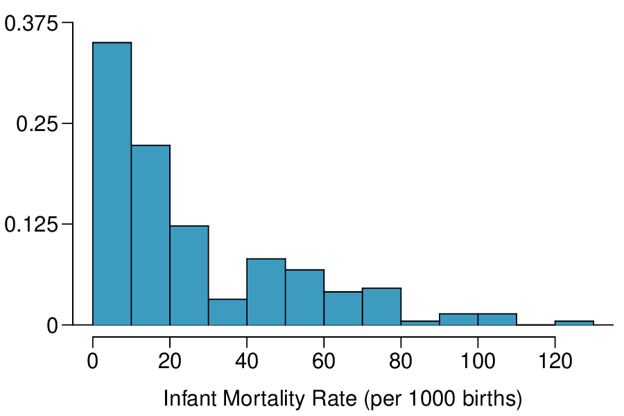
The infant mortality rate is defined as the number of infant deaths per 1,000 live births. This rate is often used as an indicator of the level of health in a country. The relative frequency histogram below shows the distribution of estimated infant death rates for 224 countries in 2014. 1
Students in an AP Statistics class were asked how many hours of television they watch per week (including online streaming). This sample yielded an average of 4.71 hours, with a standard deviation of 4.18 hours. Is the distribution of number of hours students watch television weekly symmetric? If not, what shape would you expect this distribution to have? Explain your reasoning.
No, we would expect this distribution to be right skewed. There are two reasons for this: (1) there is a natural boundary at 0 (it is not possible to watch less than 0 hours of TV), (2) the standard deviation of the distribution is very large compared to the mean.
The statistic \(\frac{\bar{x}}{median}\) can be used as a measure of skewness. Suppose we have a distribution where all observations are greater than 0, \(x_{i} \gt 0\text{.}\) What is the expected shape of the distribution under the following conditions? Explain your reasoning.
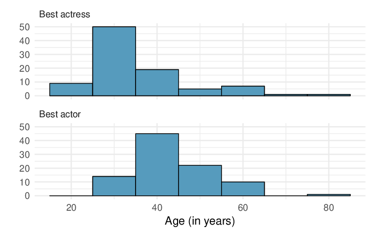
The first Oscar awards for best actor and best actress were given out in 1929. The histograms below show the age distribution for all of the best actor and best actress winners from 1929 to 2018. Summary statistics for these distributions are also provided. Compare the distributions of ages of best actor and actress winners 2
The distribution of ages of best actress winners are right skewed with a median around 30 years. The distribution of ages of best actress winners is also right skewed, though less so, with a median around 40 years. The difference between the peaks of these distributions suggest that best actress winners are typically younger than best actor winners. The ages of best actress winners are more variable than the ages of best actor winners. There are potential outliers on the higher end of both of the distributions.
The average on a history exam (scored out of 100 points) was 85, with a standard deviation of 15. Is the distribution of the scores on this exam symmetric? If not, what shape would you expect this distribution to have? Explain your reasoning.
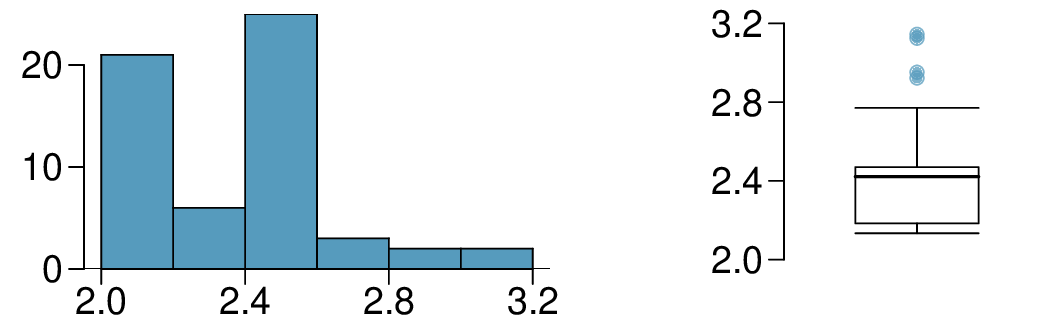
What features of the distribution are apparent in the histogram and not the box plot? What features are apparent in the box plot but not in the histogram?
In a large study of birth weight of newborns, the weights of 23,419 newborn boys were recorded. The distribution of weights was approximately normal with a mean of 7.44 lbs (3376 grams) and a standard deviation of 1.33 lbs (603 grams). The government classifies a newborn as having low birth weight if the weight is less than 5.5 pounds. 3
\(Z=\frac{10-7.44}{1.33}= 1.925\text{.}\) Using a lower bound of 2 and an upper bound of 5, we get \(P(Z \gt 1.925) = 0.027\text{.}\) Approximately 2.7% of the newborns weighed over 10 pounds.
Approximately 2.7% of the newborns weighed over 10 pounds. Because there were 23,419 of them, about \(0.027 \times 23419 \approx 632\) weighed greater than 10 pounds.
Because we have the percentile, this is the inverse problem. To get the Z-score, use the inverse normal option with 0.90 to get \(Z=1.28\text{.}\) Then solve for \(x\) in \(1.28=Z=\frac{x-7.44}{1.33}\) to get \(x=9.15\text{.}\) To be at the 90th percentile among this group, a newborn would have to weigh 9.15 pounds.
Suppose a newspaper article states that the distribution of auto insurance premiums for residents of California is approximately normal with a mean of $1,650. The article also states that 25% of California residents pay more than $1,800.
What is the \(Z\)-score that corresponds to the top 25% (or the \(75^{\text{th}}\) percentile) of the standard normal distribution?
The distribution of passenger vehicle speeds traveling on the Interstate 5 Freeway (I-5) in California is nearly normal with a mean of 72.6 miles/hour and a standard deviation of 4.78 miles/hour. 4
The speed limit on this stretch of the I-5 is 70 miles/hour. Approximate what percentage of the passenger vehicles travel above the speed limit on this stretch of the I-5.