
Advanced High School Statistics: Third Edition

Section 4.1 Sampling distribution of a sample proportion

Often, instead of the number of successes in \(n\) trials, we are interested in the proportion of successes in \(n\) trials. We can use the sampling distribution of a sample proportion to answer questions such as the following:
  • Given a fair coin, what is the probability that in 200 tosses you would get greater than 52% Tails just by random variation?
  • In a particular state, 48% support a controversial measure. When estimating the percent through polling, what is the probability that a random sample of size 200 will mistakenly estimate the percent support to be greater than 50%?

Subsection 4.1.1 The mean and standard deviation of \(\hat{p}\)

To answer these questions, we investigate the distribution of the sample proportion \(\hat{p}\text{.}\) In the last section we saw that the number of people with blood type O+ in a random sample of size 40 follows a binomial distribution with \(n=40\) and \(p=0.35\) that is centered on 14 and has standard deviation 3.0. What does the distribution of the proportion of people with blood type O+ in a sample of size 40 look like? To convert from a count to a proportion, we divide the count (i.e. number of yeses) by the sample size, \(n = 40\text{.}\) For example, 6 becomes \(8/40 = 0.20\) as a proportion and 11 becomes \(11/40 = 0.275\text{.}\)
We can find the general formula for the mean (expected value) and standard deviation of a sample proportion \(\hat{p}\) using our tools that we’ve learned so far. To get the sample mean for \(\hat{p}\text{,}\) we divide the binomial mean \(\mu_{binomial} = np\) by \(n\text{:}\)
\begin{gather*} \mu_{\hat{p}} = \frac{\mu_{binomial}}{n} = \frac{np}{n} = p \end{gather*}
As one might expect, the sample proportion \(\hat{p}\) is centered on the true proportion \(p\text{.}\) Likewise, the standard deviation of \(\hat{p}\) is equal to the standard deviation of the binomial distribution divided by \(n\text{:}\)
\begin{gather*} \sigma_{\hat{p}} = \frac{\sigma_{binomial}}{n} = \frac{\sqrt{np(1-p)}}{n} = \sqrt{\frac{p(1-p)}{n}} \end{gather*}

Mean and standard deviation of a sample proportion.

The mean and standard deviation of the sample proportion describe the center and spread of the distribution of all possible sample proportions \(\hat{p}\) from a random sample of size \(n\) with true population proportion \(p\text{.}\)
\begin{align*} \mu_{\hat{p}} \amp = p \amp \sigma_{\hat{p}}\amp = \sqrt{\frac{p(1-p)}{n}} \end{align*}
In analyses, we think of the formula for the standard deviation of a sample proportion, \(\sigma_{\hat{p}}\text{,}\) as describing the uncertainty associated with the estimate \(\hat{p}\text{.}\) That is, \(\sigma_{\hat{p}}\) can be thought of as a way to quantify the typical error in our sample estimate \(\hat{p}\) of the true proportion \(p\text{.}\) Understanding the variability of statistics such as \(\hat{p}\) is a central component in the study of statistics.
In our blood type example O+, we have \(n=40\) and \(p=0.35\text{.}\) If we look at the distribution of all possible values of a sample proportion for random samples of size 40 from this population, it is centered at \(\mu_{\hat{p}}=0.35\) and has standard deviation \(\sigma_{\hat{p}} = \sqrt{\frac{0.35(1-0.35)}{40}}=0.075\text{.}\) We see in Figure 4.1.1 that the distribution of proportion of people in a sample of size 40 with blood type O+ is equivalent to the distribution of number of people in a sample with blood type O+ of size 40, but with a change of scale. Instead of counts along the horizontal axis, we have proportions.
Figure 4.1.1. Two distributions where \(p=0.35\) and \(n=40\text{:}\) the binomial distribution for the number with blood type O+ and the sampling distribution for the proportion with blood type O+.

Example 4.1.2.

If the proportion of people in the county with blood type O+ is really 35%, find and interpret the mean and standard deviation of the sample proportion for a random sample of size 400.
Solution.
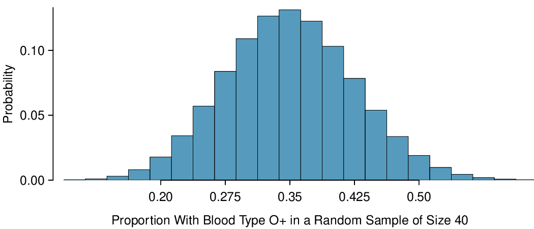
The mean of the sample proportion is the population proportion: 0.35. That is, if we took many, many samples and calculated \(\hat{p}\text{,}\) these values would average out to \(p = 0.35\text{.}\)
The standard deviation of \(\hat{p}\) is described by the standard deviation for the proportion:
\begin{gather*} \sigma_{\hat{p}} = \sqrt{\frac{p(1-p)}{n}} = \sqrt{\frac{0.35(0.65)}{400}} = 0.024 \end{gather*}
The sample proportion will typically be about 0.024 or 2.4% away from the true proportion of \(p = 0.35\text{.}\) We’ll become more rigorous about quantifying how close \(\hat{p}\) will tend to be to \(p\) in Chapter 5.

Subsection 4.1.2 The Central Limit Theorem

The distribution in Figure 4.1.1 looks an awful lot like a normal distribution. That is no nomaly; it is a result of a general principle called the Central Limit Theorem.

Central Limit Theorem and the Success-Failure Condition.

When observations are independent and the sample size is sufficiently large, the sample proportion \(\hat{p}\) will tend to follow a normal distribution with the following mean and standard deviation:
\begin{align*} \mu_{\hat{p}} \amp = p \amp \sigma_{\hat{p}}\amp = \sqrt{\frac{p(1-p)}{n}} \end{align*}
In order for the Central Limit Theorem to hold, the sample size is typically considered sufficiently large when \(np \geq 10\) and \(n(1-p) \geq 10\text{,}\) which is called the success-failure condition.
The Central Limit Theorem is incredibly important, and it provides a foundation for much of statistics. As we begin applying the Central Limit Theorem, be mindful of the two technical conditions: the observations must be independent, and the sample size must be sufficiently large such that \(np \geq 10\) and \(n(1-p) \geq 10\text{.}\)

How To Verify Sample Observations Are Independent.

If the observations are from a random process such as tossing a coin, then they are independent.
If the observations are from a random sample with replacement, then they are independent.
If the observations are from a simple random sample (without replacement), we can treat them as independent if the sample size is less than 10% of the population size.
If a sample is from a seemingly random process, e.g. an occasional error on an assembly line, checking independence is more difficult. In this case, use your best judgement.
When the sample exceeds 10% of the population size, the methods we discuss tend to overestimate the sampling error slightly versus what we would get using more advanced methods.
 1 
For example, we could use what’s called the finite population correction factor: if the sample is of size \(n\) and the population size is \(N\text{,}\) then we can multiple the typical standard deviation formula by \(\sqrt{\frac{N-n}{n-1}}\) to obtain a smaller, more precise estimate of the actual standard deviation. When \(n \lt 0.1 \times N\text{,}\) this correction factor is relatively close to 1.
An interesting question to answer is, what happens when \(np \lt 10\) or \(n(1-p) \lt 10\)? We can simulate drawing samples of different sizes where, say, the true proportion is \(p = 0.25\text{.}\) Here’s a sample of size 10:
no no yes yes no no no no no no
In this sample, we observe a sample proportion of yeses of \(\hat{p}=\frac{2}{10}=0.2\text{.}\) We can simulate many such proportions to understand the sampling distribution for \(\hat{p}\) when \(n = 10\) and \(p = 0.25\text{,}\) which we’ve plotted in Figure 4.1.4 alongside a normal distribution with the same mean and variability. These distributions have a number of important differences.
Table 4.1.3.
Unimodal? Smooth? Symmetric?
Normal: \(N(0.25,10.14)\) YES YES YES
\(n=10\text{,}\)\(p=0.25\) YES NO NO
Notice that the success-failure condition was not satisfied when \(n = 10\) and \(p = 0.25\text{:}\)
\begin{align*} np = 10 \times 0.25 - 2.5 \amp \amp n(1-p)=10 \times 0.75 = 7.5 \end{align*}
This single sampling distribution does not show that the success-failure condition is the perfect guideline, but we have found that the guideline did correctly identify that a normal distribution might not be appropriate.
Figure 4.1.4. Left: simulations of \(\hat{p}\) when the sample size is \(n = 10\) and the population proportion is \(p = 0.25\text{.}\) Right: a normal distribution with the same mean (0.25) and standard deviation (0.137).
We can complete several additional simulations, shown in Figure 4.1.5 and Figure 4.1.6, and we can see some trends:
  1. When either \(np\) or \(n(1 − p)\) is small, the distribution is more discrete, i.e. not continuous.
  2. When \(np\) or \(n(1 − p)\) is smaller than 10, the skew in the distribution is more noteworthy.
  3. The larger both \(np\) and \(n(1 − p)\text{,}\) the more normal the distribution. This may be a little harder to see for the larger sample size in these plots as the variability also becomes much smaller.
  4. When \(np\) and \(n(1 − p)\) are both very large, the distribution’s discreteness is hardly evident, and the distribution looks much more like a normal distribution.
So far we’ve only focused on the skew and discreteness of the distributions. We haven’t considered how the mean and standard error of the distributions change. Take a moment to look back at the graphs, and pay attention to three things:
  1. The centers of the distribution are always at the population proportion, \(p\text{,}\) that was used to generate the simulation. Because the sampling distribution for \(\hat{p}\) is always centered at the population parameter \(p\text{,}\) it means the sample proportion \(\hat{p}\) is unbiased when the data are independent and drawn from such a population.
  2. For a particular population proportion \(p\text{,}\) the variability in the sampling distribution decreases as the sample size \(n\) becomes larger. This will likely align with your intuition: an estimate based on a larger sample size will tend to be more accurate.
  3. For a particular sample size, the variability will be largest when \(p = 0.5\text{.}\) The differences may be a little subtle, so take a close look. This reflects the role of the proportion \(p\) in the standard error formula: \(SE=\sqrt{\frac{p(1-p)}{n}}\text{.}\) The standard error is largest when \(p = 0.5\text{.}\)
At no point will the distribution of \(\hat{p}\) look perfectly normal, since \(\hat{p}\) will always be take discrete values \((x/n)\text{.}\) It is always a matter of degree, and we will use the standard success-failure condition with minimums of 10 for \(np\) and \(n(1 − p)\) as our guideline within this book.

Three Important Factors About The Distribution Of A Sample Proportion \(\hat{p}\).

When the observations can be considered independent, such as from a random sample of less than 10% of the population, the distribution of the sample proportion can be described as follows.
  1. CENTER: The mean of a sample proportion is \(p\text{.}\)
  2. SPREAD: The SD of a sample proportion is \(\sqrt{\frac{p(1-p)}{n}}\text{.}\)
  3. SHAPE: When \(np \geq 10\) and \(n(1-p) \geq 10\text{,}\) the sample proportion closely follows a normal distribution.
Using these facts, we can now answer the question posed at the beginning of this section.
Figure 4.1.5. Sampling distributions for several scenarios of \(p\) and \(n\text{.}\) Rows: \(p = 0.10\text{,}\) \(p = 0.20\text{,}\) \(p = 0.50\text{,}\) \(p = 0.80\text{,}\) and \(p = 0.90\text{.}\) Columns: \(n = 10\) and \(n = 25\text{.}\)
Figure 4.1.6. Sampling distributions for several scenarios of \(p\) and \(n\text{.}\) Rows: \(p = 0.10\text{,}\) \(p = 0.20\text{,}\) \(p = 0.50\text{,}\) \(p = 0.80\text{,}\) and \(p = 0.90\text{.}\) Columns: \(n = 50\text{,}\) \(n = 100\text{,}\) and \(n = 250\text{.}\)

Subsection 4.1.3 Normal approximation for the distribution of \(\hat{p}\)

Example 4.1.7.

Find the probability that less than 30% of a random sample of 400 people will be blood type O+ if the population proportion is 35%.
Solution.
In the previous section we verified that \(np\) and \(n(1-p)\) are at least 10. The mean of the sample proportion is 0.35 and the standard deviation for the sample proportion is given by \(\sqrt{\frac{0.35(1-0.35)}{400}}=0.024\text{.}\) We can find a Z-score and use our calculator to find the probability:
\begin{align*} Z \amp = \frac{\hat{p} - \mu_{\hat{p}}}{\sigma_{\hat{p}}} = \frac{0.30 - 0.35}{0.024} = -2.1\\ P(\amp Z \lt -2.1) = 0.0179 \end{align*}
We leave it to the reader to construct a figure for this example.

Example 4.1.8.

The probability 0.0179 is the same probability we calculated when we found the probability of getting fewer than 120 with blood type O+ out of 400! Why is this?
Solution.
Notice that \(120/400=0.30\text{.}\) Using the binomial distribution to find the probability of fewer than 120 with blood type O+ in the sample is equivalent to using the distribution of \(\hat{p}\) to find the probability of a sample proportion less than 0.30.

Guided Practice 4.1.9.

Given a population that is 50% male, what is the probability that a sample of size 200 would have greater than 55% males? Remember to verify that conditions for normal approximation are met.
 2 
First, verify the conditions: There is a random sample, and the sample size is much smaller than the population size, so observations can be considered independent. Also, \(np = 200(0.5) = 100 \ge 10\) and \(n(1- p) = 200(0.5) = 100 \ge 10\text{,}\) so the normal approximation is reasonable. Next we find the mean and standard deviation of \(\hat{p}\text{:}\) \(\mu_{\hat{p}} = p =0.50\) and\(\sigma_{\hat{p}} = \sqrt{\frac{p(1-p)}{n}} =\sqrt{\frac{0.5(0.5)}{200}} = 0.0354\text{.}\) Then we find the \(Z\)-score and find the upper tail of the normal distribution: \(Z=\frac{\hat{p}-\mu_{\hat{p}}}{\sigma_{\hat{p}}}= \frac{0.55-0.5}{0.0354}=1.412 \rightarrow P(Z>1.412)=0.07\text{.}\) The probability of getting a sample proportion of 55% or greater is about 0.07.

Subsection 4.1.4 Section summary

  • A Z-score represents the number of standard deviations a value in a data set is above or below the mean. To calculate a Z-score use: \(Z=\frac{x-\text{mean}}{\text{SD}}\text{.}\)
  • The standard deviation of \(\hat{p}\) describes the typical error or distance of the sample proportion from the population proportion. It also tells us how much the sample proportion is likely to vary from one random sample to another.
  • The sampling distribution for the sample proportion \(\hat{p}\) for a random sample of size \(n\) is identical to the binomial distribution with parameters \(n\) and \(\text{,}\) but with a change of scale, i.e. different mean and different SD, but same shape.
  • The same success-failure condition for the binomial distribution holds for a sample proportion \(\hat{p}\text{.}\)
  • Three important facts about the sampling distribution of the sample proportion \(\hat{p}\text{:}\)
    • The mean of a sample proportion is denoted by \(\mu_{\hat{p}}\text{,}\) and it is equal to \(p\text{.}\) (center)
    • The SD of a sample proportion is denoted by \(\sigma_{\hat{p}}\text{,}\) and it is equal to \(\sqrt{\frac{p(1-p)}{n}}\text{.}\) (spread)
    • When \(np\ge 10\) and \(n(1-p)\ge 10\text{,}\) the distribution of the sample proportion will be approximately normal. (shape)
  • We use these properties when solving the following type of normal approximation problem involving a sample proportion. Find the probability of getting more / less than % yeses in a sample of size \(n\).
    1. Identify \(n\) and \(p\text{.}\) Verify than \(np\ge 10\) and \(n(1-p)\ge 10\text{,}\) which implies that normal approximation is reasonable.
    2. Calculate the Z-score. Use \(\mu_{\hat{p}} = p\) and \(\sigma_{\hat{p}} = \sqrt{\frac{p(1-p)}{n}}\) to standardize the sample proportion.
    3. Find the appropriate area under the normal curve.

Exercises 4.1.5 Exercises

1. Distribution of \(\hat{p}\).

Suppose the true population proportion were \(p = 0.95\text{.}\) The figure below shows what the distribution of a sample proportion looks like when the sample size is \(n = 20\text{,}\) \(n = 100\text{,}\) and \(n = 500\text{.}\) (a) What does each point (observation) in each of the samples represent? (b) Describe the distribution of the sample proportion, \(\hat{p}\text{.}\) How does the distribution of the sample proportion change as \(n\) becomes larger?
Solution.
  1. Each observation in each of the distributions represents the sample proportion (\(\hat{p}\)) from samples of size \(n = 20\text{,}\) \(n = 100\text{,}\) and \(n = 500\text{,}\) respectively.
  2. The centers for all three distributions are at 0.95, the true population parameter. When \(n\) is small, the distribution is skewed to the left and not smooth. As n increases, the variability of the distribution (standard deviation) decreases, and the shape of the distribution becomes more unimodal and symmetric.

2. Distribution of \(\hat{p}\).

Suppose the true population proportion were \(p = 0.5\text{.}\) The figure below shows what the distribution of a sample proportion looks like when the sample size is \(n = 20\text{,}\) \(n = 100\text{,}\) and \(n = 500\text{.}\) What does each point (observation) in each of the samples represent? Describe how the distribution of the sample proportion, \(\hat{p}\text{,}\) changes as \(n\) becomes larger.

3. Vegetarian college students.

Suppose that 8% of college students are vegetarians. Determine if the following statements are true or false, and explain your reasoning.
  1. The distribution of the sample proportions of vegetarians in random samples of size 60 is approximately normal since \(n \ge 30\text{.}\)
  2. The distribution of the sample proportions of vegetarian college students in random samples of size 50 is right skewed.
  3. A random sample of 125 college students where 12% are vegetarians would be considered unusual.
  4. A random sample of 250 college students where 12% are vegetarians would be considered unusual.
  5. The standard error would be reduced by one-half if we increased the sample size from 125 to 250.
Solution.
  1. False. Doesn’t satisfy success-failure condition.
  2. True. The success-failure condition is not satisfied. In most samples we would expect \(\hat{p}\) to be close to 0.08, the true population proportion. While \(\hat{p}\) can be much above 0.08, it is bound below by 0, suggesting it would take on a right skewed shape. Plotting the sampling distribution would confirm this suspicion.
  3. False. \(SE_{\hat{p}} = 0.0243\text{,}\) and \(\hat{p} = 0.12\) is only \(\frac{0.12-0.08}{0.0243} = 1.65\) SEs away from the mean, which would not be considered unusual.
  4. True. \(\hat{p} = 0.12\) is 2.32 standard errors away from the mean, which is often considered unusual.
  5. False. Decreases the SE by a factor of \(1/ \sqrt{2}\text{.}\)

4. Young Americans, Part I.

About 77% of young adults think they can achieve the American dream. Determine if the following statements are true or false, and explain your reasoning.
 3 
A. Vaughn. “Poll finds young adults optimistic, but not about money”. In: Los Angeles Times (2011).
  1. The distribution of sample proportions of young Americans who think they can achieve the American dream in samples of size 20 is left skewed.
  2. The distribution of sample proportions of young Americans who think they can achieve the American dream in random samples of size 40 is approximately normal since \(n \ge 30\text{.}\)
  3. A random sample of 60 young Americans where 85% think they can achieve the American dream would be considered unusual.
  4. A random sample of 120 young Americans where 85% think they can achieve the American dream would be considered unusual.

5. Distribution of \(\hat{p}\).

Suppose the true population proportion were \(p = 0.5\) and a researcher takes a simple random sample of size \(n=50\text{.}\)
  1. Find and interpret the standard deviation of the sample proportion \(\hat{p}\text{.}\)
  2. Calculate the probability that the sample proportion will be larger than 0.55 for a random sample of size 50.
Solution.
  1. \(SD_{\hat{p}} = \sqrt{p(1 - p)/n} = 0.0707\text{.}\) This describes the typical distance that the sample proportion will deviate from the true proportion, \(p = 0.5\text{.}\)
  2. \(\hat{p}\) approximately follows \(N(0.5, 0.0707)\text{.}\) \(Z = (0.55 - 0.50)/0.0707 \approx 0.71\text{.}\) This corresponds to an upper tail of about 0.2389. That is, \(P(\hat{p} > 0.55) \approx 0.24\text{.}\)

6. Distribution of\(\hat{p}\).

Suppose the true population proportion were \(p = 0.6\) and a researcher takes a simple random sample of size \(n=50\text{.}\)
  1. Find and interpret the standard deviation of the sample proportion \(\hat{p}\text{.}\)
  2. Calculate the probability that the sample proportion will be larger than 0.65 for a random sample of size 50.

7. Nearsighted children.

It is believed that nearsightedness affects about 8% of all children. We are interested in finding the probability that fewer than 12 out of 200 randomly sampled children will be nearsighted.
  1. Estimate this probability using the normal approximation to the binomial distribution.
  2. Estimate this probability using the distribution of the sample proportion.
  3. How do your answers from parts (a) and (b) compare?
Solution.
  1. First we need to check that the necessary conditions are met. There are \(200 \times 0.08 = 16 \) expected successes and \(200 \times (1 - 0.08) = 184\) expected failures, therefore the success-failure condition is met. Then the binomial distribution can be approximated by \(N(\mu = 16, \sigma = 3.84)\text{.}\) \(P(X \lt 12) = P(Z \lt -1.04) = 0.1492\text{.}\)
  2. Since the success-failure condition is met the sampling distribution of \(\hat{p} ~ N(\mu = 0.08, \sigma = 0.0192)\text{.}\) \(P(\hat{p} \lt 0.06)= P(Z \lt -1.04) = 0.1492\)
  3. As expected, the two answers are the same.

8. Social network use.

The Pew Research Center estimates that as of January 2014, 89% of 18-29 year olds in the United States use social networking sites.
 4 
Pew Research Center, Washington, D.C. Social Networking Fact Sheet, accessed on May 9, 2015.
Calculate the probability that at least 95% of 500 randomly sampled 18-29 year olds use social networking sites.

9. CLT for proportions, Part 1.

Define the term “sampling distribution” of the sample proportion, and describe how the shape, center, and spread of the sampling distribution change as the sample size increases when \(p = 0.1\text{.}\)
Solution.
The sampling distribution is the distribution of sample proportions from samples of the same size randomly sampled from the same population. As the same size increases, the shape of the sampling distribution (when \(p = 0.1\)) will go from being rightskewed to being more symmetric and resembling the normal distribution. With larger sample sizes, the spread of the sampling distribution gets smaller. Regardless of the sample size, the center of the sampling distribution is equal to the true mean of that population, provided the sampling isn’t biased

10. CLT for proportions, Part 2.

Define the term “sampling distribution” of the sample proportion, and describe how the shape, center, and spread of the sampling distribution change as the sample size increases when \(p = 0.8\text{.}\)
You have attempted of activities on this page.