Exercise 8.2.10.10 presents regression output from a model for predicting the heart weight (in g) of cats from their body weight (in kg). The coefficients are estimated using a dataset of 144 domestic cat. The model output is also provided below.
We see that the point estimate for the slope is positive. What are the hypotheses for evaluating whether body weight is positively associated with heart weight in cats?
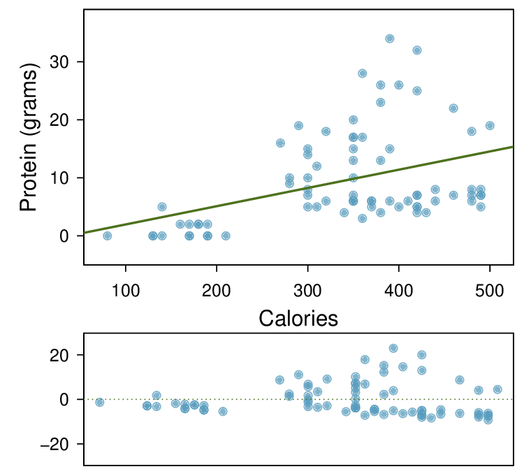
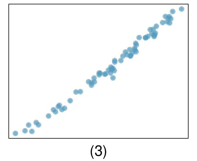
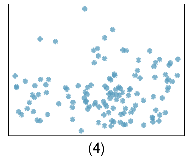
Exercise 8.2.10.6 introduced a data set on nutrition information on Starbucks food menu items. Based on the scatterplot and the residual plot provided, describe the relationship between the protein content and calories of these menu items, and determine if a simple linear model is appropriate to predict amount of protein from the number of calories.
There is an upwards trend. However, the variability is higher for higher calorie counts, and it looks like there might be two clusters of observations above and below the line on the right, so we should be cautious about fitting a linear model to these data.
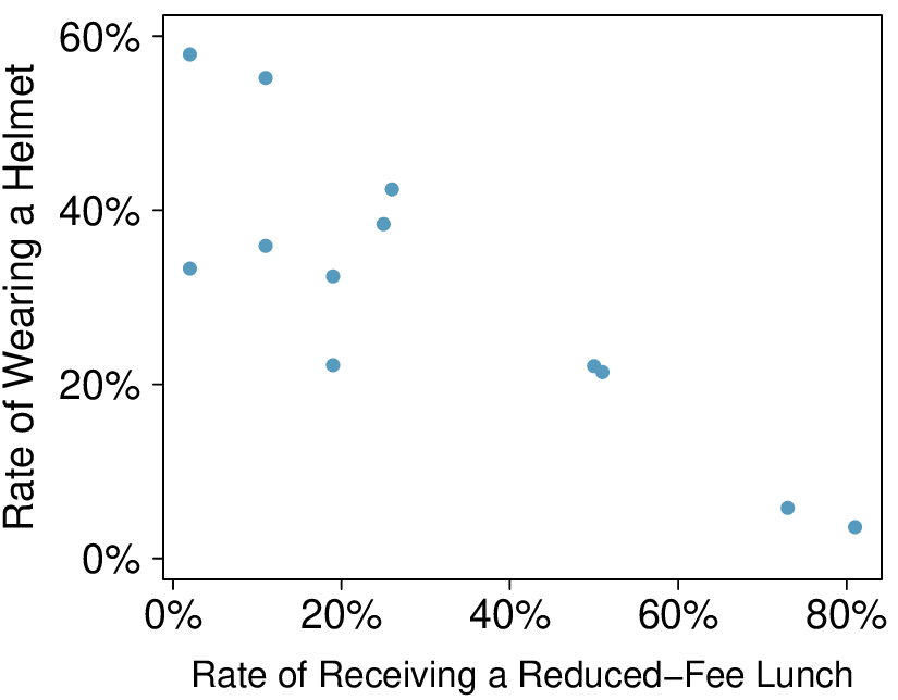
The scatterplot shows the relationship between socioeconomic status measured as the percentage of children in a neighborhood receiving reduced-fee lunches at school (lunch) and the percentage of bike riders in the neighborhood wearing helmets (helmet). The average percentage of children receiving reduced-fee lunches is 30.8% with a standard deviation of 26.7% and the average percentage of bike riders wearing helmets is 38.8% with a standard deviation of 16.9%.
What would the value of the residual be for a neighborhood where 40% of the children receive reduced-fee lunches and 40% of the bike riders wear helmets? Interpret the meaning of this residual in the context of the application.
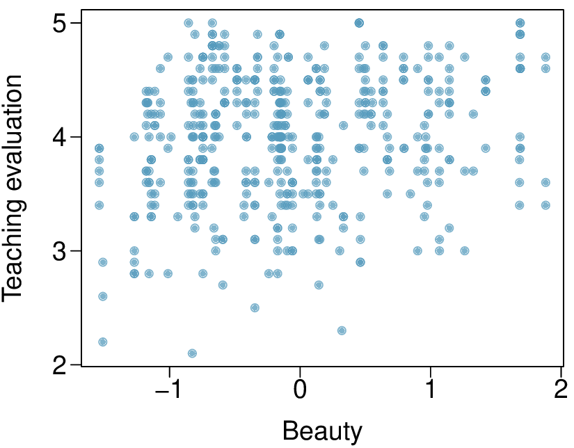
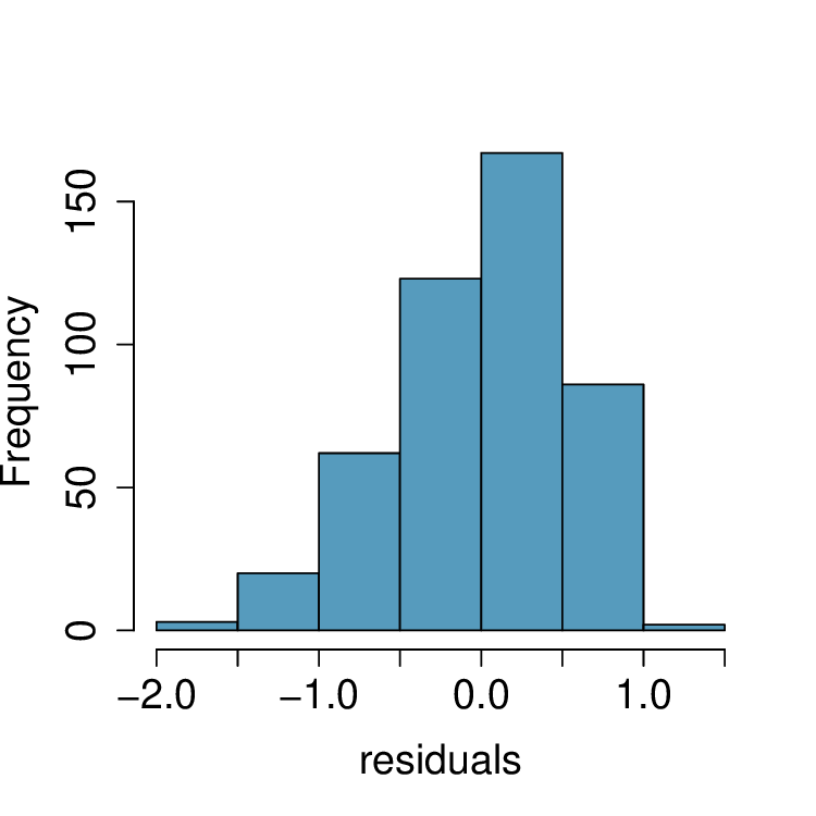
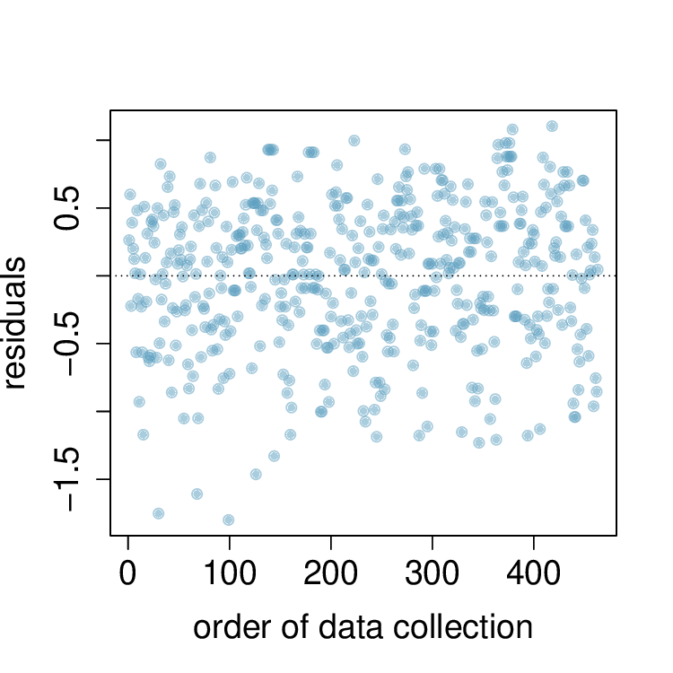
Many college courses conclude by giving students the opportunity to evaluate the course and the instructor anonymously. However, the use of these student evaluations as an indicator of course quality and teaching effectiveness is often criticized because these measures may reflect the infuence of non-teaching related characteristics, such as the physical appearance of the instructor. Researchers at University of Texas, Austin collected data on teaching evaluation score (higher score means better) and standardized beauty score (a score of 0 means average, negative score means below average, and a positive score means above average) for a sample of 463 professors. 1
Daniel S Hamermesh and Amy Parker. “Beauty in the classroom: Instructors’ pulchritude and putative pedagogical productivity”. In: Economics of Education Review 24.4 (2005), pp. 369-376.
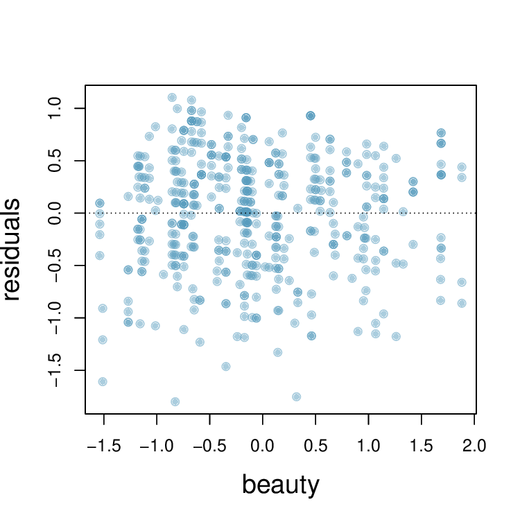
The scatterplot below shows the relationship between these variables, and regression output is provided for predicting teaching evaluation score from beauty score.
Given that the average standardized beauty score is -0.0883 and average teaching evaluation score is 3.9983, calculate the slope. Alternatively, the slope may be computed using just the information provided in the model summary table.
Do these data provide convincing evidence that the slope of the relationship between teaching evaluation and beauty is positive? Explain your reasoning.
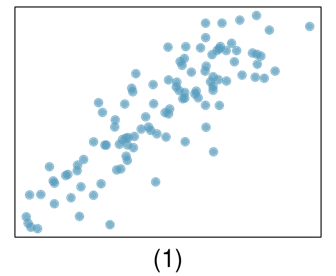
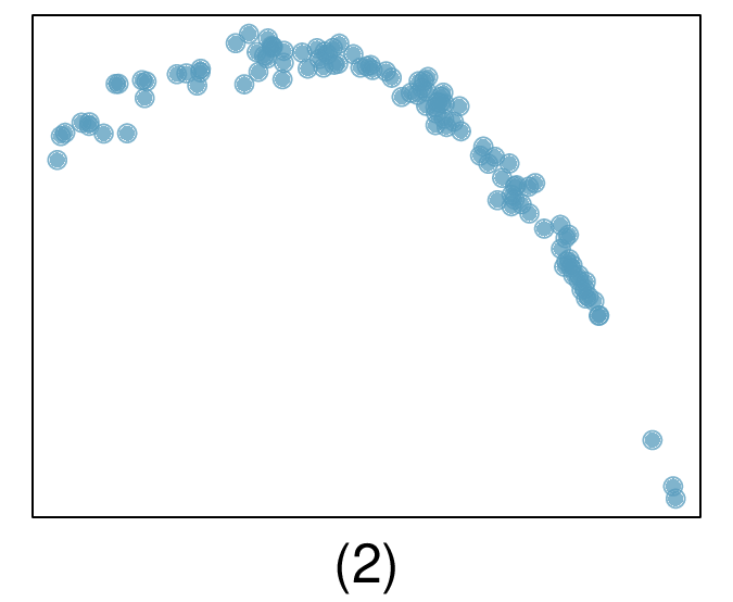
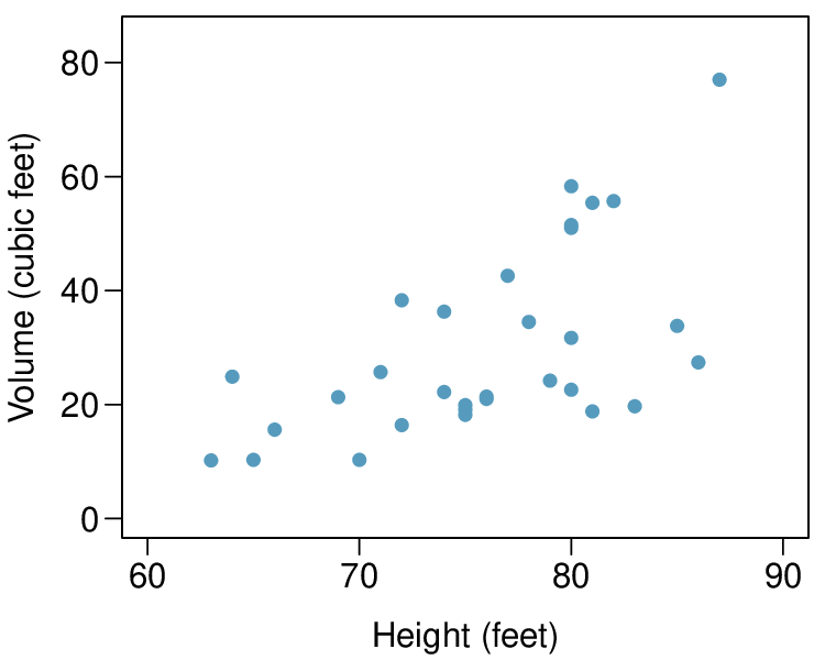
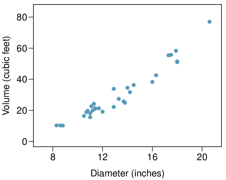
The scatterplots below show the relationship between height, diameter, and volume of timber in 31 felled black cherry trees. The diameter of the tree is measured 4.5 feet above the ground. 2
Suppose you have height and diameter measurements for another black cherry tree. Which of these variables would be preferable to use to predict the volume of timber in this tree using a simple linear regression model? Explain your reasoning.
There is a weak-to-moderate, positive, linear association between height and volume. There also appears to be some non-constant variance since the volume of trees is more variable for taller trees.
Since the relationship is stronger between volume and diameter, using diameter would be preferred. However, as mentioned in part (b), the relationship between volume and diameter may not be, and so we may benefit from a model that properly accounts for nonlinearity.