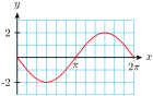
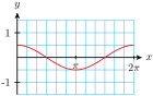
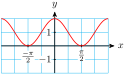
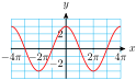
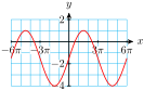
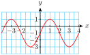
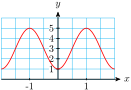
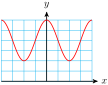
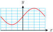
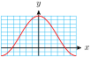
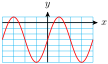
In Chapter 4 we saw that the amplitude, period, and midline of a sinusoidal graph are determined by the coefficients in its formula. The circular functions (sine and cosine of real numbers) behave the same way.
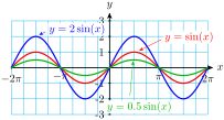
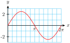
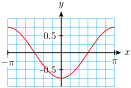
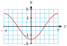
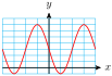
All three graphs have the same period (\(2\pi\)) and midline (\(y=0\)), but the graph of \(f\) has amplitude 2, and the graph of \(g\) has amplitude 0.5.
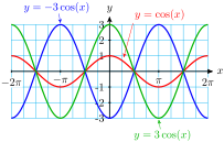
The amplitude of \(~y=A\sin (t)~\) is given by \(\abs A\text{,}\) and the same is true of \(~y=A\cos (t)\text{.}\) In the next exercise, remember that the amplitude is always a nonnegative number.
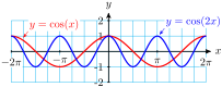
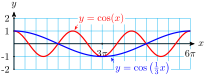
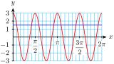
Both graphs have the same amplitude (\(1\)) and midline (\(y=0\)), but the graph of \(f\) completes two cycles from \(0\) to \(2\pi\) instead of one. The period of \(~f(x)=\cos (\alert{2}x)~\) is \(\dfrac{2\pi}{\alert{2}}=\pi\text{.}\)
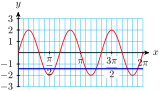
The graph of \(~g(x)=\cos \left(\alert{\dfrac{1}{3}}x\right)~\) completes one cycle between \(0\) and \(6\pi\text{.}\) Its period is \(\dfrac{2\pi}{\alert{\frac{1}{3}}}=6\pi\text{.}\)
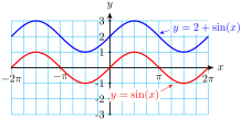
Each point on the graph of \(~f(x)=2+\sin (x)~\) has \(y\)-coordinate 2 units higher than the corresponding point on the graph of \(~y=\sin (x)~\text{.}\) Thus, the graph of \(~f(x)=2+\sin (x)~\) is shifted vertically by 2 units relative to the graph of \(~y=\sin (x)~\text{.}\) In particular, the midline of \(~f(x)=\alert{2}+\sin (x)~\) is the line \(y=\alert{2}\text{.}\)
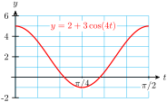
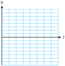
One way to make a quick sketch of a sinusoidal graph is to use a table of values. The trick is to choose convenient values for the input variable. In the table below, notice that we choose the quadrantal angles as the input values for the trigonometric function.
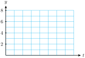
Notice from the table that the graph completes one cycle from \(t=0\) to \(t=\dfrac{\pi}{2}\text{,}\) which confirms that the period is \(\dfrac{\pi}{2}\text{.}\) Finally, we plot the points \((t,y)\) from the table, and use them as "guidepoints" to sketch a sinusoidal graph, as shown below.
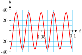
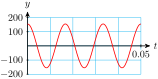
Sinusoidal functions are used to model a great variety of physical phenomena, including sound and light waves, tides and planetary orbits, and the life cycles of plants and animals. They are also often used to approximate periodic functions that are not exactly sinusoidal, such as blood pressure.
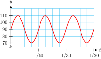
A typical blood pressure for a healthy adult, measured in millimeters of mercury, varies between 70 and 110, and a typical heart rate is 60 beats per minute. Write a sinusoidal function that approximates blood pressure, and sketch its graph.
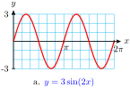
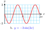
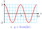
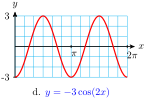
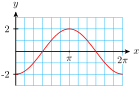
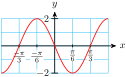
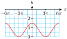
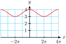
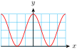
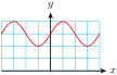
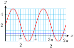
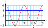
In the preceding Example, we could have chosen either a sine or a cosine function to model blood pressure; both describe the periodic behavior described. However, if we are given, or would like to specify, the starting point for a sinusoidal function, one choice can be more suitable than the other. Consider the functions graphed below.
The graph in (c) is modeled by a cosine, because it starts at the maximum point, and the graph in (d) starts at the minimum point, so we choose a negative cosine to model it.
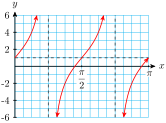
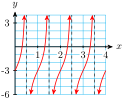
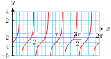
The transformations of shifting and stretching can be applied to the tangent function as well. The graph of \(~y=\tan x~\) does not have an amplitude, but we can see any vertical stretch by comparing the function values at the guidepoints.
Recall that the period of the tangent function is \(\pi\text{.}\) We make a table of values for one cycle of the function, choosing multiples of \(\dfrac{\pi}{4}\) as the inputs for the tangent function. Then we plot the guidepoints, and sketch a tangent function through them. The graph is shown below.
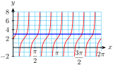
we see that the graph is stretched vertically by a factor of \(A=3\text{.}\) The midline is \(y=1\text{,}\) so the graph is shifted up by 1 unit. Finally, the coefficient \(B=2\) compresses the graph horizontally by a factor of 2, so the period of the graph is \(\dfrac{\pi}{2}\text{,}\) and there are four cycles between \(0\) and \(2\pi\)
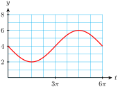
Changes to the amplitude, period, and midline of the basic sine and cosine graphs are called transformations. Changing the midline shifts the graph vertically, changing the amplitude stretches or compresses the graph vertically, and changing the period stretches or compresses the graph horizontally.
Transformationhe maximum value of a certain sinusoidal function is \(M\text{,}\) and its minimum value is \(m\text{.}\) What is the midline of the function? What is its amplitude?
In Problems 9–16, we use transformations to sketch graphs of the functions in Problems 1–8. Sketch one cycle of each graph by hand and label scales on the axes.
The height of the tide in Cabot Cove can be approximated by a sinusoidal function. At 5 am on July 23, the water level reached its high mark at the 20-foot line on the pier, and at 11 am, the water level was at its lowest at the 4-foot line.
The population of mosquitoes at Marsh Lake is a sinusoidal function of time. The population peaks around June 1 at about 6000 mosquitoes per square kilometer, and is smallest on December 1, at 1000 mosquitoes per square kilometer.
The paddlewheel on the Delta Queen steamboat is 28 feet in diameter, and is rotating once every ten seconds. The bottom of the paddlewheel is 4 feet below the surface of the water.
The ship’s logo is painted on one of the paddlewheel blades. At \(t=0\text{,}\) the blade with the logo is at the top of the wheel. Sketch a graph of the logo’s heightabove the water as a function of \(t\text{.}\)
Delbert’s bicycle wheel is 24 inches in diameter, and he has a light attached to the spokes 10 inches from the center of the wheel. It is dark, and he is cycling home slowly from work. The bicycle wheel makes one revolution every second.
At \(t=0\text{,}\) the light is at its highest point the bicycle wheel. Sketch a graph of the light’s height as a function of \(t\text{.}\)
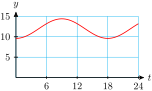
The number of hours of daylight in Salt Lake City varies from a minimum of 9.6 hours on the winter solstice to a maximum of 14.4 hours on the summer solstice. Time is measured in months, starting at the winter solstice.
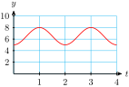
A weight is 6.5 feet above the floor, suspended from the ceiling by a spring. The weight is pulled down to 5 feet above the floor and released, rising past 6.5 feet in 0.5 second before attaining its maximum height of 8 feet. The weight oscillates between its minimum and maximum height.
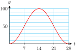
Although the moon is spherical, what we see from earth looks like a disk, sometimes only partly visible. The percentage of the moon’s disk that is visible varies between 0 (at new moon) to 100 (at full moon), over a 28-day cycle.