Imagine that you are riding on a Ferris wheel. As the wheel turns, your height above the ground increases and then decreases again, repeating the same pattern each time the Ferris wheel makes a complete rotation. This pattern is an example of a periodic function. We use periodic functions to model phenomena that exhibit cyclical behavior, such as the height of tides, seasonal patterns of growth in plants and animals, radio waves, and planetary motion.
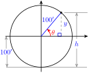
We’ll create a mathematical model for a ride on a Ferris wheel that has a radius of 100 feet and rotates counterclockwise. Our model will be a function that describes your height above the ground as you ride the wheel. In order to graph the Ferris wheel function, we must first specify the input and output variables, and then choose a coordinate system to display their values.
We’ll place the origin at the center of the Ferris wheel. Then the line from the origin to your position on the wheel makes an angle with the horizontal, as shown at right. This angle, \(\theta\text{,}\) will be the input variable for the function. Your height, \(h\text{,}\) is also a variable, and is related to the \(y\)-coordinate of your position; in fact, we see that \(h = y + 100\text{,}\) because the center of the wheel is 100 feet above the ground.
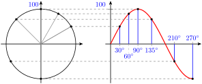
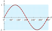
To simplify the model, we’ll first graph \(y\) as the output variable, instead of \(h\text{.}\) As the angle \(\theta\) increases from \(0\degree\) to \(90\degree\text{,}\) your \(y\)-coordinate increases from 0 to 100. You are then at the top of the wheel. Then, as \(\theta\) increases from \(90\degree\) to \(180\degree\text{,}\) your \(y\)-coordinate decreases from 100 back to 0.
Finally, as \(\theta\) increases from \(180\degree\) to \(360\degree\text{,}\) your \(y\)-coordinate decreases from 0 to \(-100\) and then increases from \(-100\) back to 0. You have made one complete rotation on the Ferris wheel. If you go around again, \(\theta\) increases from \(360\degree\) to \(720\degree\text{,}\) and the graph of your \(y\)-coordinate will repeat the pattern of the first rotation. The figure above shows how your \(y\)-coordinate is plotted as a function of the angle \(\theta\text{.}\)
Our Ferris wheel model used values of \(\sin (\theta)\text{,}\) so let us explore its properties. Remember that the trigonometric ratio \(\sin (\theta)\) is actually a function of the angle \(\theta\text{.}\) Thus, for each value of \(\theta\text{,}\) there is only one value of \(\sin (\theta)\text{,}\) and we may write \(f(\theta) = \sin (\theta)\text{.}\)
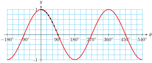
Plot the points in the table and connect them with a smooth curve to graph the sine function in the first quadrant, from \(0\degree\) to \(90\degree\text{.}\)
Recall that the values of \(\sin (\theta)\) in the second quadrant can be found using reference angles: \(\sin (180\degree - \theta) = \sin (\theta)\text{.}\) This fact gives us values of \(\sin \theta\) from \(90\degree\) to \(180\degree\text{.}\)
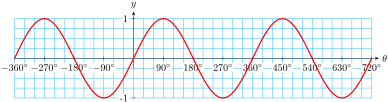
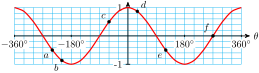
If we continue the graph for angles larger than \(360\degree\) or smaller than \(0\degree\text{,}\) we find that the same pattern repeats, as shown below. This should not be surprising, because we know that coterminal angles have the same trigonometric ratios.
The sine is an example of a periodic function. The smallest interval on which the graph repeats is called the period of the graph. From the graph in the previous example, we make the following observations:
The distance between the midline and either the maximum or minimum value is called the amplitude of the function, so the amplitude of the sine function is 1.
and pressing ZOOM\(7\) for the trig window. The graph shows two periods of the sine function, from \(\theta = -360\degree\) to \(\theta = 360\degree\text{.}\)
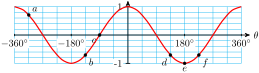
In the previous exercise you graphed the height of a person riding on a Ferris wheel. Your graph involved \(\sin (\theta)\text{,}\) because the sine function tells us the \(y\)-coordinate of a point that travels around a circle. The cosine function tells us the \(x\)-coordinate of a point that travels around a circle.
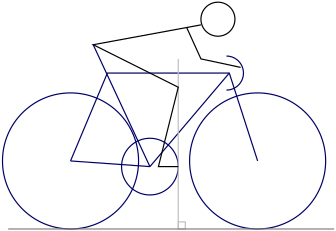
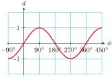
Small adjustments to the fit of a bicycle can affect both the cyclist’s efficiency and the stress on his or her joints. The KOPS rule (Knee Over Pedal Stem) aligns the cyclist’s knee directly over the pedal at the point of maximum force, as shown at right. As the cyclist’s foot rotates away from this KOPS line, stress on the knee increases.
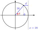
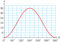
Suppose the pedal crank is 18 centimeters long. When the crank makes an angle \(\theta\) with the horizontal, how far is the cyclist’s foot displaced horizontally from the KOPS line?
The cyclist’s foot travels around a circle of radius 18 centimeters. If we place the origin at the center of the chain gear, the \(x\)-coordinate of the foot is given by
\begin{equation*}
x = r \cos (\theta) = 18 \cos (\theta)
\end{equation*}
(See the figure at right.) The KOPS line is the vertical line \(x = 18\text{,}\) so the horizontal distance between the cyclist’s foot and the KOPS line is
\begin{equation*}
d = 18 - 18 \cos (\theta)
\end{equation*}
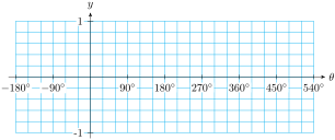
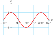
Complete the table below with values rounded to two decimal places. Use the table and your knowledge of reference angles to graph the cosine function, \(~f(\theta) = \cos (\theta),~\) from \(-180\degree\) to \(540\degree\text{.}\)
Use your graph to find the period, amplitude, and midline of the cosine function. How does the graph of cosine differ from the graph of sine? (Hint: Consider the intercepts of the graph, and the location of the maximum and minimum values.)
Period: \(360\degree\text{,}\) amplitude: \(1\text{,}\) midline: \(y = 0\text{.}\) The cosine graph starts \((\theta = 0\degree)\) at its high point, while the sine graph starts \((\theta = 0\degree)\) at its midline.
Perhaps it is time to review our use of function notation. Recall that we use the notation \(~y = f(x)~\) to indicate that \(y\) is a function of \(x\text{,}\) that is, \(x\) is the input variable and \(y\) is the output variable.
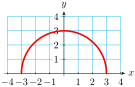
We choose several values for the input variable, \(x\text{,}\) and evaluate the function to find the corresponding values of the output variable, \(y\text{.}\) For example,
Of course, we don’t always use \(x\) and \(y\) for the input and output variables. In the previous example, we could write \(~w = f(t) = \sqrt{9 - t^2}~\) for the function, so that \(t\) is the input and \(w\) is the output. The table of values and the graph are the same; only the names of the variables have changed.
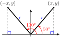
When we discuss trigonometric functions, there are several variables involved. Our definitions of the trig ratios involve four variables: \(x\text{,}\)\(y\text{,}\)\(r\text{,}\) and \(\theta\text{,}\) as illustrated below.
If the value of \(r\) is fixed for a given situation, such as the Ferris wheel or the bicycle wheel discussed above, then \(x\) and \(y\) are both functions of \(\theta\text{.}\) This means that the values of \(x\) and \(y\) depend only on the value of the angle \(\theta\text{.}\) If \(r = 1\text{,}\) we have
\begin{align*}
x \amp = f(\theta) = \cos (\theta)\\
y \amp = g(\theta) = \sin (\theta)
\end{align*}
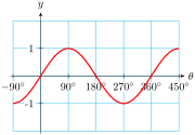
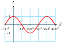
The graphs of these functions are shown below. Note particularly that the horizontal axis displays values of the input variable, and the vertical axis displays the output variable.
If we use different variables for the input and output, the functions and their graphs are the same, but the axes should be labeled with the appropriate variables.
A common mistake is to think of \(\cos (\theta)\) as a product, cos times\(\theta\text{,}\) but this makes no sense, because "cos" by itself has no meaning. Remember that \(\cos (\theta)\) represents a single number, namely the output of the cosine function.
The tangent function is periodic, but its graph is not similar to the graphs of sine and cosine. Recall that the tangent of an angle in standard position is defined by
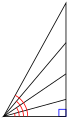
Study the figure at right to see that as \(\theta\) increases from \(0\degree\) to \(90\degree\text{,}\)\(y\) increases while \(x\) remains constant, so the value of \(\tan (\theta)\) increases.
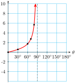
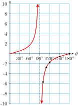
As \(\theta\) gets closer to \(90\degree\text{,}\)\(\tan (\theta)\) increases very rapidly. Recall that \(\tan (90\degree)\) is undefined, so there is no point on the graph at \(\theta = 90\degree\text{.}\) The graph of \(f(\theta) = \tan (\theta)\) for \(0\le\theta\lt 90\degree\) is shown at right.
In particular, for values of \(\theta\) close to \(90\degree\text{,}\) the values of \(\tan (\theta)\) are large negative numbers. We plot several points and sketch the graph in the second quadrant.
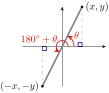
Now let’s consider the graph of \(f(\theta) = \tan (\theta)\) in the third and fourth quadrants. The tangent is positive in the third quadrant, and negative in the fourth quadrant. In fact, from the figure below you can see that the angles \(\theta\) and \(180\degree + \theta\) are vertical angles.
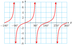
Thus, the graph of \(\tan (\theta)\) in the third quadrant is the same as its graph in the first quadrant. Similarly, the graph of the tangent function in the fourth quadrant is the same as its graph in the second quadrant. The completed graph is shown below.
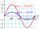
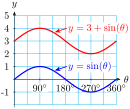
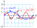
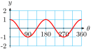
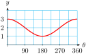
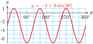
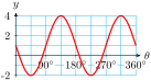
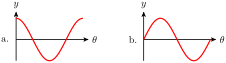
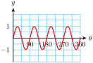
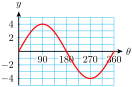
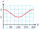
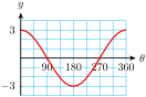
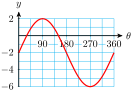
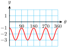
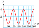
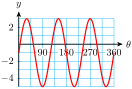
All sine and cosine graphs have the characteristic "wave" shape we’ve seen in previous examples. But we can alter the size and frequency of the waves by changing the formula for the function. In the next example we consider three variations of the sine function.
We plot the points, and connect them with a sine-shaped wave. Compare the graph, shown at right, to the graph of \(y = \sin (\theta)\text{.}\) The graph is like a sine graph, except that it oscillates between a maximum value of \(3\) and a minimum value of \(-3\text{.}\) The amplitude of this function is \(3\text{.}\)
This graph has the same amplitude as \(y = \sin (\theta)\text{,}\) but the entire graph is shifted up by \(3\) units, as shown at right. The midline of this function is the line \(y = 3\text{.}\)
You can continue the table for \(\theta\) between \(180\degree\) and \(360\degree\text{,}\) and plot the points to find the graph shown at right. The graph has the same amplitude and midline as \(y = \sin (\theta)\text{,}\) but it completes three cycles from \(0\degree\) to \(360\degree\) instead of one cycle. The period of this graph is one-third of \(360\degree\text{,}\) or \(120\degree\text{.}\)
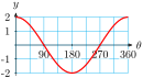
The quantities \(A, B,\) and \(k\) in the equations above are called parameters, and their values for a particular function give us information about its graph.
For this function, \(A = 4,~ B = 3,\) and \(k = -3\text{.}\) Its amplitude is \(4\text{,}\) its period is \(\dfrac{360\degree}{3} = 120\degree\text{,}\) and its midline is \(y = -3\text{.}\) The graph is shown below.
We use the notation \(y = f(x)\) to indicate that \(y\) is a function of \(x\text{,}\) that is, \(x\) is the input variable and \(y\) is the output variable.
The period of the sine function is \(360\degree\text{.}\) Its midline is the horizontal line \(y = 0\text{,}\) and the amplitude of the sine function is 1.
The graph of the cosine function has the same period, midline, and amplitude as the graph of the sine function. However, the locations of the intercepts and of the maximum and minimum values are different.
The tangent function has period \(180\degree\text{.}\) It is undefined at odd multiples of \(90\degree\text{,}\) and is increasing on each interval of its domain.
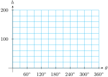
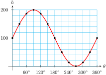
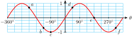
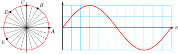
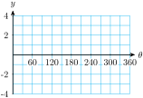
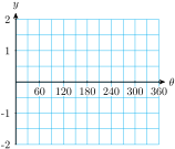
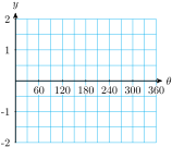
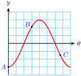
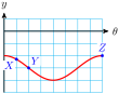
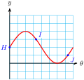
The graph shows your height as a function of angle as you ride the Ferris wheel. For each location \(A\)–\(E\) on the Ferris wheel, mark the corresponding point on the graph.
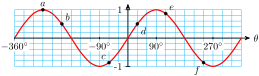
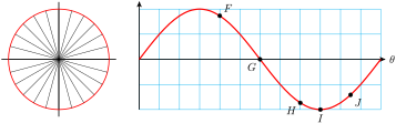
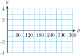
The graph shows your height as a function of angle as you ride the Ferris wheel. For each location \(F\)–\(J\) on the graph, mark the corresponding point on the Ferris wheel.
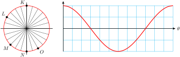
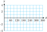
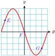
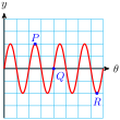
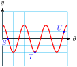
The graph shows the horizontal displacement of your foot from the center of the chain gear as you pedal a bicycle. For each location \(K\)–\(O\) on the chain gear, mark the corresponding point on the graph.
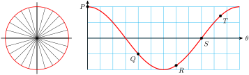
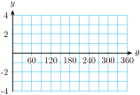
The graph shows the horizontal displacement of your foot from the center of the chain gear as you pedal a bicycle. For each location \(P\)–\(T\) on the graph, mark the corresponding point on the chain gear.