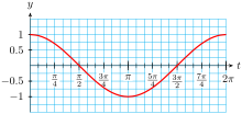
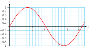
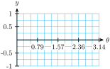
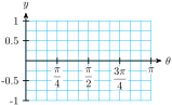
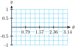
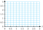
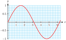
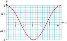
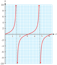
We can graph the circular functions \(~y =\sin (t),~ y = \cos (t),\) and \(y = \tan (t) ~\) just as we graphed trigonometric functions of angles in degrees. The only difference is that we scale the horizontal axis in radians.
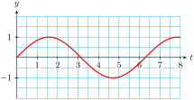
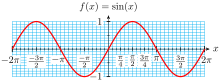
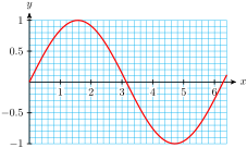
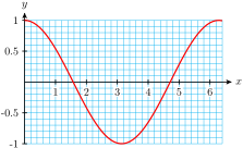
You can probably recognize this graph as one cycle of \(y = \sin (t)\text{.}\) For example, you can see that the graph completes one cycle at \(t = 2\pi\) radians, or approximately 6.28. It reaches its maximum value, \(y = 1\text{,}\) at \(t = \dfrac{\pi}{2}\text{,}\) or approximately 1.57. You should also notice that \(y = 0\) at \(t = \pi\text{,}\) approximately 3.14.
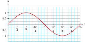
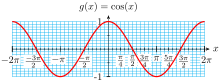
Instead of scaling the horizontal axis with integers, we often use multiples of \(\pi\text{.}\) Using such a scale, we can show the exact location of the intercepts of the graph, and of its high and low points.
We start by making a table of values for \(\sin (t)\text{,}\) where \(t\) is in radians. We’ll use the special values of \(t\text{,}\) because we know the sines of those values.
In order to plot the points in the table, we scale the horizontal axis in multiples of \(\dfrac{\pi}{12}\text{.}\) (Note that the special values are all multiples of \(\dfrac{\pi}{12}\text{.}\) Thus, \(~\dfrac{\pi}{6} = 2\left(\dfrac{\pi}{12}\right)\text{,}\)\(~ \dfrac{\pi}{4} = 3\left(\dfrac{\pi}{12}\right)\text{,}\) and so on.) The table lists values of \(\sin (t)\) in the first two quadrants; in quadrants three and four the sine values are negative.
If we continued to plot points for values of \(t\) greater than \(2 \pi\) or less than 0, we would see the periodic behavior of the graph, as it repeats the same shape over each interval of length \(2 \pi\text{,}\) just as it does for periods of \(360\degree\) when the angles are measured in degrees.
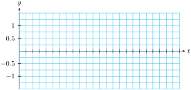
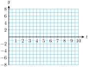
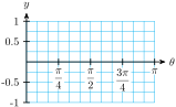
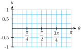
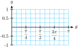
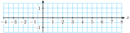
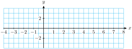
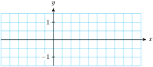
Because we know the basic shapes of the sine and cosine graphs, to make an adequate graph it is usually sufficient to plot the guide points at the quadrantal angles, and then draw a smooth curve through the points. Try it for yourself. Use the axes below.
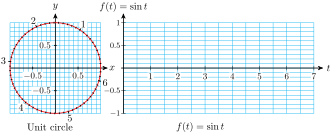
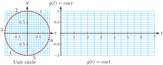
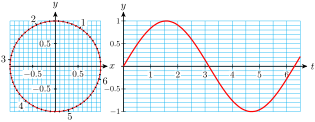
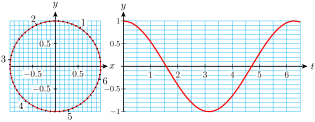
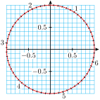
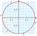
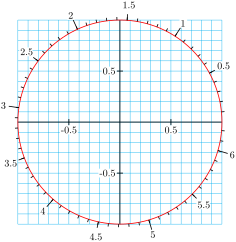
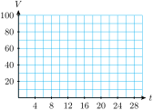
We are going to graph \(~f(t) = \sin (t)~\) and \(~g(t) = \cos (t)~\) from their definitions. The unit circle \(~x^2 + y^2 = 1~\) at the left of each grid is marked off in radians. (Each tick mark is \(0.1\) radian.) The horizontal \(t\)-axis of each grid is also marked in radians.
At the value of \(t\) you chose in step 1, lightly draw a vertical line segment the same length as the \(y\)-coordinate of \(P\text{.}\) Put a dot at the top (or bottom) of the line segment.
At the value of \(t\) you chose in step 1, lightly draw a vertical line segment the same length as the \(x\)-coordinate of \(P\text{.}\) Put a dot at the top (or bottom) of the line segment.
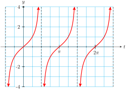
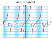
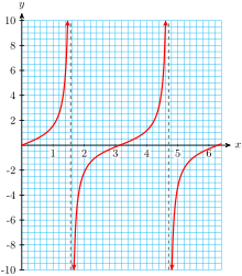
Finally, we consider the graph of the tangent function. Once again, the only difference between this new graph and our old version of the tangent graph in degrees is that the horizontal axis is scaled in radians.
We plot the points and connect them with smooth curves, remembering that \(\tan \left(\dfrac{\pi}{2}\right)\) is undefined. The graph repeats for values of \(t\) between \(\pi\) and \(2\pi\text{,}\) and we will include \(t\)-values outside the table in order to show three periods.
While the graph in degrees had vertical asymptotes at \(~\theta = \pm 90\degree~\) and \(~\theta = 270\degree\text{,}\) this graph has vertical asymptotes at \(~t = \pm\dfrac{\pi}{2}~\) and \(~t = \dfrac{3\pi}{2}\text{.}\)
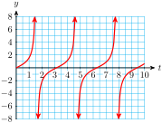
Sketch a graph of the tangent function \(y =\tan (t)\) and scale the horizontal axis in integers, as shown below. Label the \(t\)-intercepts and the vertical asymptotes with their coordinates.
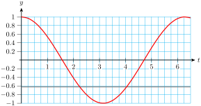
The figure shows a graph of \(~y = \cos (t)\text{,}\) with \(t\) in radians, and the horizontal line \(y = -0.62\text{.}\) The solutions of the equation are the \(t\)-coordinates of the intersection points, and these appear to be about \(t = 2.25\) and slightly over \(4.0\text{,}\) perhaps \(4.05\text{.}\) You can check that these values roughly satisfy the equation; it is difficult to read the graph with any greater accuracy.
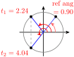
The cosine is negative in the second and third quadrants, so we expect to find our answers between \(t = 1.57\) and \(t = 4.71\text{.}\) We use a calculator to find one of the angles:
Rounded to hundredths, the second quadrant angle is \(t_1 = 2.24\) radans. To find the other angle, we first find the reference angle for \(t_1\text{:}\)
All angles coterminal with \(t_1\) and \(t_2 \) are also solutions of the equation \(~~\cos t = -0.62~~\text{.}\) So adding or subtracting multiples of \(2 \pi\) to \(t_1\) and \(t_2 \) produces all the solutions. For example, \(2.24 + 2\pi = 8.52\) and \(4.04 - 2 \pi = -2.24\) are solutions.
Because \(~\tan \left(\dfrac{\pi}{4}\right) = 1\text{,}\) one of the solutions is \(t_1 = \dfrac{\pi}{4}\text{.}\) Remember that \(\tan (t)\) repeats every \(\pi\) units. All other solutions of the equation \(\tan t = 1\) can be found by adding (or subtracting) multiples of \(\pi\) to these two solutions. We write the solutions as
\begin{equation*}
t = \dfrac{\pi}{4} + k \pi ~~ \text{where } k \text{ is an integer.}
\end{equation*}
Now that we have defined trigonometric functions of real numbers, we can describe periodic phenomena as functions of time (or other variables besides angles).
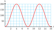
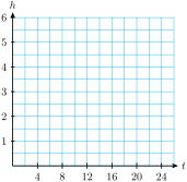
For example, we began this chapter with a Ferris wheel of radius 100 feet that rotates once every 8 minutes. If you board the Ferris wheel at the bottom, your height is given as a function of time by
The graph of \(h = f(t)\) is shown above. From the graph, we see that the midline of the function is \(h = 100\text{,}\) its amplitude is 100, and its period is 8 (which is reasonable because the Ferris wheel rotates every 8 minutes). You can review period, midline, and amplitude of periodic functions in Section 4.3.
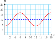
From the graph, we see that \(D(t) \lt 8\) for \(t\) between 0 and 2, or in January and February. \(D(t)\) is also less than 8 for a short time between \(t = 11\) and \(t = 12\text{,}\) at the end of December.
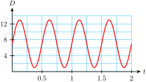
The pistons in an automobile engine move up and down in the cylinders. If \(t\) is in milliseconds, the distance from the top of the piston to the top of the cylinder is given in centimeters by
\begin{equation*}
D = 7 + 6\sin (4\pi t)
\end{equation*}
The domain of a function is the set of all possible input values. For many familiar functions, the domain is the set of all real numbers. In particular, the domain of any linear or quadratic function is the set of all real numbers.
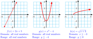
Consider the functions \(~f(x) = 2x + 5~\) and \(~g(x) = x^2 - 4~\) shown below. We can use any real number as an input for either of these functions, and their graphs extend across the entire \(x\)-axis.
However, for other types of functions we must sometimes exclude certain values from the domain. For example, the domain of the function \(~h(x) = \sqrt{x + 3}~\) is restricted because we cannot take the square root of a negative number. We must have \(x + 3 \ge 0\text{,}\) so the domain of the function consists of all \(x \ge -3\text{.}\)
You can see the domain of a function in its graph; notice that there are no points on the graph of \(~h(x) = \sqrt{x + 3}~\) with \(x\)-coordinates less than \(-3\text{.}\)
The range of a function is the set of all output values for the function. We can also see the range of a function in its graph; it is the set of all \(y\)-values for points on the graph.
Because the graph of \(~f(x) = 2x + 5~\) extends infinitely in both directions, its range consists of all real numbers. There is an input value that will produce any output we want.
However, the range of \(~g(x) = x^2 - 4~\) consists of all \(y \ge -4\text{,}\) because there are no points on the graph with \(y\)-coordinate less than \(-4\text{.}\)
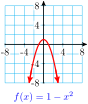
There are no restrictions on the input values for this function, so its domain is all real numbers. The graph is a parabola with high point at \((0,1)\text{,}\) so the range of the function is all \(y \le 1\text{.}\) See the figure below left.
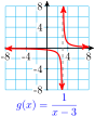
Because we cannot divide by zero, we cannot allow \(x = 3\) for this function. Thus, the domain of \(g\) is all real numbers except \(3\text{.}\) The graph has a horizontal asymptote at \(y = 0\text{,}\) and you can see that there is no input that will produce an output of zero. So the range of \(g\) is all real numbers except \(0\text{.}\)
What about the domain and range of the trigonometric functions? The sine and cosine both include all real numbers in their domains; we can find the sine or cosine of any number. Because the output values of the sine and cosine are both defined by the coordinates of points on a unit circle, their values cannot be greater than \(1\) or less than \(-1\text{.}\) The range of both sine and cosine is the interval \([-1,1]\text{.}\)
The tangent function is undefined at odd multiples of \(\dfrac{\pi}{2}\) (that is, at \(\cdots,~ \dfrac{-3\pi}{2},~ \dfrac{-\pi}{2},~ \dfrac{\pi}{2},~ \dfrac{3\pi}{2},~\cdots\)), so those values must be excluded from its domain. However, the output values of the tangent function increase without bound as the input approaches \(\dfrac{\pi}{2}\) from the left, and decrease from the right. The range of the tangent is all real numbers.
We can use a graph to solve trigonometric equations, or the inverse trig keys on a calculator or computer. We can find exact values for the solutions of equations involving the special values without using a calculator.
For each equation below, suppose that \(\omega\) is one of the solutions between \(0\) and \(2\pi\text{.}\) Use the diagram to find the other solution.
For Problems 45–52, use your calculator in radian mode. In part (a), evaluate the trigonometric function, and in part (b), find all solutions between \(0\) and \(\dfrac{\pi}{2}\text{.}\) Round your answers to two decimal places.
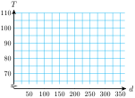
When observed from earth, the moon looks like a disk that is partially visible and partially in shadow. The percentage of the disk that is visible can be approximated by
Label on your graph the points that correspond to full moon, half moon, and new moon. (New moon occurs when the part of the moon receiving sunlight is facing directly away from the earth.)
A weight is suspended from the ceiling on a spring. The weight is pushed straight up, compressing the spring, then released. The height of the weight above the ground is given by the function
For Problems 63–66, the figure shows an arc of length \(t\text{,}\) and the coordinates of its terminal point. Find the terminal point of each related arc given below, and give its sine, cosine, and tangent.
Locate the four values \(t,~ 2\pi - t,~ \pi - t,~ \) and \(\pi + t\) from Problem 63 on the graph of \(f(t) = \sin (t)\text{,}\) on the graph of \(g(t) = \cos (t)\text{,}\) and on the graph of \(h(t) = \tan (t)\) shown below.