The Cartesian coordinate system is also called the rectangular coordinate system, because it describes a location in the plane as the vertex of a rectangle. To construct a rectangular coordinate system, we begin with two perpendicular axes that intersect at the origin. The \(x\)- and \(y\)-coordinates of a point indicate the length and width of a rectangle with one vertex at the origin. The point \(P(x,y)\) sits at the opposite vertex of the rectangle, as shown in the figure below.
In Chapter 9 we used vectors to specify a location by giving a distance and a direction. For example, we might say that the airport is located 5 miles southwest of the city center. This method of designating locations is so useful that we will construct a new coordinate system using the same tools: distance and direction.
In the polar coordinate system we start with the origin or pole, and a single ray from the pole, called the polar axis. We describe the location of a point \(P\) in the plane by measuring the distance, \(\abs{r}\text{,}\) from \(P\) to the pole, and the angle, \(\theta\text{,}\) that \(\vec{OP}\) makes with the polar axis (measured counterclockwise). The components of the ordered pair \((r, \theta)\) are called the polar coordinates of the point \(P\text{.}\)
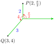
In our work with polar coordinates, we will always use radians for the angle \(\theta\text{.}\) For example, the point \(P\left(2, \dfrac{\pi}{2}\right)\) is located 2 units from the pole at an angle of \(\dfrac{\pi}{2}\) radians, and \(Q(3,4)\) is located 3 units from the pole at an angle of 4 radians. The graphs of \(P\) and \(Q\) are shown at right.
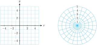
A piece of graph paper in rectangular coordinates consists of a grid of horizontal and vertical lines. These are the lines \(x=k\) and \(y=k\text{,}\) for evenly spaced values of \(k\text{.}\) Each vertical grid line consists of points that have the same \(x\)-coordinate, and each horizontal grid line is made up of points that have the same \(y\)-coordinate. The grid lines are bench marks to help us locate points with specific rectangular coordinates.
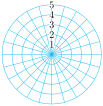
A piece of graph paper in polar coordinates consists of a grid of concentric circles and radial lines, as shown below. Each circle consists of points with the same \(r\)-coordinate; they are all the same distance from the pole. All points with the same \(\theta\)-coordinate lie on one of the radial lines. This grid helps us locate points with specific polar coordinates.
You are used to thinking in rectangular coordinates: to locate a point, we move so many units left or right, and so many units up or down. When working in polar coordinates, we want to "think radially:" how far to move from the pole, and in which direction.
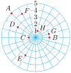
To plot point \(A\text{,}\) we move 1 unit away from the pole in the direction \(\dfrac{\pi}{2}\text{,}\) as shown at right. To plot point \(B\text{,}\) we move 2 units away from the pole in the direction \(\dfrac{7\pi}{4}\text{.}\)
Note that even though the independent or input variable in polar coordinates is nearly always \(\theta\text{,}\) it is customary to list the dependent or output variable first: \((r, \theta)\text{.}\)
Each point has infinitely many polar coordinates, because we can add multiples of \(2\pi\) to the value of \(\theta\text{.}\) For example, the point with polar coordinates \(\left(1, \dfrac{\pi}{2}\right)\) also has polar coordinates \(\left(1,\dfrac{5\pi}{2}\right)\) and \(\left(1, \dfrac{-3\pi}{2}\right)\text{.}\)
If we allow negative values of \(r\text{,}\) there are even more ways to write the coordinates of a point. Each angle designates a line through the pole, and each line has both a postive and a negative direction.
On the line at \(\theta = \dfrac{\pi}{4}\text{,}\) for instance, the positive direction lies in the first quadrant, so that the point \((2, \dfrac{\pi}{4})\) is designated by \(P\) in the figure at right. To plot the point \((-2, \dfrac{\pi}{4})\text{,}\) we move in the opposite direction from the pole, arriving at point \(Q\text{.}\) Note that the point \(Q\) can also be designated by the coordinates \((2, \dfrac{5\pi}{4})\text{.}\)
The point \(S(2,\pi)\) is also \((-2,\pi)\) or \((-2,0)\text{.}\) The point \(T\left(3, \dfrac{2\pi}{3}\right)\) can also be designated by \(\left(-3, \dfrac{2\pi}{3}+\pi\right)\text{,}\) or \(\left(-3, \dfrac{5\pi}{3}\right)\text{.}\)
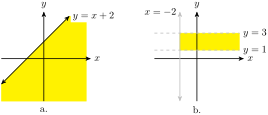
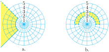
In Cartesian coordinates, we use equations and inequalities to describe regions in the plane. For example, the shaded region in figure (a) is the graph of \(y \le x+2\text{.}\) The pair of inequalities \(x \ge -2,~ 1 \lt y \lt 3\) describes the region in figure (b). This region is particularly simple, in that its boundaries are portions of the coordinate grid lines \(x=k\) and \(y=k\text{,}\) where \(k\) is a constant.
In the polar plane, the coordinate grid lines are circles centered at the pole, with equations \(r=k\text{,}\) and lines through the pole, with equations \(\theta=k\text{.}\)
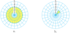
The region consists of all points between 1 (inclusive) and 3 units from the pole. No restriction is given on \(\theta\text{,}\) so the region is the annular ring shown in figure (a).
The region includes all points up to 2 units from the pole, but only between the lines \(\theta = \dfrac{\pi}{6}\) and \(\theta = \dfrac{\pi}{3}\text{.}\) These curves bound the pie-shaped wedge (circular sector) shown in figure (b).
SubsectionConverting Between Polar and Cartesian Coordinates
Using trigonometry, it is easy to convert from polar coordinates to Cartesian, or vice versa. The figure below shows how the two sets of coordinates are related.
To find the angle \(\theta\text{,}\) it is not enough to compute \(\tan^{-1}\left(\dfrac{y}{x}\right)\text{;}\) we must choose the angle in the same quadrant as the given point.
There are infinitely many values of \(\theta\) that satisfy this equation, but our point lies in the third quadrant, so we take \(\theta = \dfrac{4\pi}{3}\text{.}\)
You can check that the polar coordinates \(\left(1,\dfrac{4\pi}{3}\right)\) convert back to Cartesian coordinates \(\left(-\dfrac{1}{2},-\dfrac{\sqrt{3}}{2}\right)\text{.}\)
In the previous Example, the angle \(\theta\) is not given by \(\tan^{-1}(\sqrt{3}) = \dfrac{\pi}{3}\text{,}\) because the given point lies in the third quadrant. Remember that there are always two angles between \(0\) and \(2\pi\) with a given tangent.
Polar coordinates are useful for studying objects or phenomena that have radial symmetry, such as circles, spheres, and cylinders, or the central forces (those that act equally in all directions), such as gravity and electric charge. The equations describing these objects are often simpler in polar coordinates than they are in Cartesian coordinates.
It is not hard to convert an equation from Cartesian to polar coordinates: we replace each \(x\) with \(r\cos (\theta)\) and each \(y\) with \(r\sin(\theta)\text{.}\)
Neither of these equations is simpler than the Cartesian version, but that should not surprise us, because the original equation describes a line, and Cartesian coordinates are better suited to rectilinear graphs.
Perhaps you recognize the equation in the previous exercise as a circle. Note also that its polar equation has a simpler form than the familiar Cartesian version.
Converting equations from polar to Cartesian form is not as straightforward as the other direction (and is sometimes impossible). Here are some strategies to try:
Expressions of the form \(r\cos (\theta)\) or \(r\sin (\theta)\) can be replaced by \(x\) and \(y\text{,}\) respectively.
In the polar plane, the coordinate grid lines are circles centered at the pole, with equations \(r=k\text{,}\) and lines through the pole, with equations \(\theta = k\text{.}\)
To convert an equation from Cartesian to polar coordinates, we replace each \(x\) with \(r\cos (\theta)\) and each with \(y\) with \(r\sin (\theta)\text{.}\) To convert an equation from polar to Cartesian coordinates, look for expressions of the form \(r\cos (\theta),~r\sin (\theta),~r^2\text{,}\) or \(\tan (\theta)\text{.}\)
For Problems 25–32, convert the Cartesian coordinates to polar coordinates with \(r \ge 0\) and \(0 \le \theta \le 2\pi\text{.}\) Give exact values for \(r\) and \(\theta\text{.}\)