Section C.1 Quick References

πŸ“

Worksheet Basics

✳️ Differential Equations and their Components.

Differential Equation (DE)
An equation that involves one or more derivatives of an unknown function.
Variables
The dependent variable represents the unknown function that you are solving for and always has derivatives applied to it. The dependent variable is a function of the independent variable. In
\begin{gather*} 12y'' + (x+5)y' - \ln(x) y = 5 - \cos x\text{,} \end{gather*}
dependent \(\leftarrow y\quad\) & \(\quad\) independent \(\leftarrow x\text{.}\)
Terms & Free Terms
Parts of an equation separated by \(+\text{,}\) \(-\text{,}\) or \(=\) and each containing a different form of the dependent variable. The collection of all terms without a dependent variable is referred to as a free term.
\begin{gather*} \us{\large y'' \text{ term}}{\boxed{12y''}} + \us{\large y' \text{ term}}{\boxed{(x+5)y'}} - \us{\large y \text{ term}}{\boxed{\ln(x) y}} = \us{\large\text{free term}}{\boxed{5 - \cos x}} \end{gather*}
Coefficients
The part of a term multiplied by the dependent variable or its derivatives.
\begin{gather*} \boxed{12}\us{\Large y'',\ y',\ y \text{ coefficients}}{\us{\nwarrow}{\ y}'' + \us{\uparrow}{\boxed{(x+5)}}\ y' \us{\nearrow}{-\ }} \boxed{\ln (x)}\ y = 5 - \cos x \end{gather*}

✳️ Order & Linearity.

Order
The highest order derivative present in a DE.
Linear Term
A term of the form:
\begin{equation*} a(t)\ y,\ a(t)\ y',\ a(t)\ y'',\ a(t)\ y''',\ \ldots\text{,} \end{equation*}
where \(y\) is the dependent variable, and \(a(t)\) is a coefficient that depends only on the independent variable \(t\text{.}\)
Linear DE
A DE composed entirely of linear terms.
Nonlinear DE
A DE that contains at least one nonlinear term.

Worksheet Solutions to Differential Equations

✳️ Solutions & Initial Conditions.

Satisfying a DE
A function satisfies a DE if substituting it into the dependent variable results in the equation simplifying to a true statement (e.g., \(0 = 0\)).
Solution
A function that satisfies the DE.
General Solution
The common form (template) of all the solutions in the family. It contains constants that can take any value.
Particular Solution
A single solution obtained by assigning specific values to the constants in the general solution.
Family of Solutions
The collection of all possible particular solutions.
Initial Conditions
Known values of the solution or its derivatives at a specific point, used to determine a particular solution from the general solution.

✳️ Direct Integration.

Direct Integration
A method to solve differential equations of the form:
\begin{equation*} \frac{d}{dx}\left[g(x,y)\right] = f(x), \end{equation*}
by integrating both sides with respect to the independent variable \(x\text{.}\)

Worksheet Separation of Variables

✳️ First-Order Differential Equations.

First-Order Differential Equation
Every first-order differential equation can be written in the form
\begin{equation*} f(x, y, y') = 0\text{.} \end{equation*}
This just means that all the terms in the equation have been moved to the left-hand side, which can only contain the independent variable, \(x\text{,}\) the dependent variable, \(y\text{,}\) and its derivative, \(y'\text{.}\)

✳️ Separation of Variables.

First-Order Separable Differential Equation
These equations can be written as:
\begin{equation*} \frac{dy}{dx} = f(x) \cdot g(y). \end{equation*}
Separation of Variables Method
A solution technique for separable equations. It involves isolating \(y\) and \(x\) terms on opposite sides, followed by integration.

Worksheet Integrating Factor

✳️ Integrating Factor.

First-Order Linear Differential Equation
These equations take the standard form:
\begin{equation*} y' + P(x)y = Q(x). \end{equation*}
Integrating Factor
A function, \(\mu\text{,}\) multiplied onto the standard form, above, to reverse the product rule, leading to the equation, \(\mu' = P\mu\text{,}\) with the solution
\begin{equation*} \mu = e^{\int P(x) dx}. \end{equation*}
Integrating Factor Method
A solution method for first-order linear equations that uses an integrating factor to convert the equation into a form solvable by direct integration.

Worksheet Qualitative Methods

✳️ Slope Fields & Autonomous Equations.

Slope Field
A picture of the slopes that a solution curve must follow at each point of the plane, drawn as short segments. It represents the entire family of solutions to \(y' = f(t, y)\text{;}\) here \(f(t, y)\) is the β€œslope generator” that outputs the required slope at any point \((t, y)\text{.}\)
Autonomous Equation
A first-order equation that contains no explicit \(t\text{,}\) so the rate of change of \(y\) depends only on \(y\) itself:
\begin{equation*} \frac{dy}{dt} = f(y). \end{equation*}
Its slope field looks β€œstriped”: horizontal shifts of a solution are again solutions.

✳️ Equilibria & the Phase Line.

Equilibrium Solution
A constant solution \(y(t) = c\) where the slope is zero. Found by solving the algebraic equation
\begin{equation*} f(c) = 0. \end{equation*}
A solution that starts at an equilibrium stays there forever.
Phase Line
A compressed, one-dimensional summary of an autonomous slope field drawn on a vertical \(y\)-axis: equilibria are marked with solid dots, regions where \(f(y) > 0\) get upward arrows, and regions where \(f(y) < 0\) get downward arrows.
Stability Classification
Each equilibrium is one of three types, according to how nearby solutions behave:
  • Stable (sink): solutions move toward the equilibrium from both sides.
  • Unstable (source): solutions move away from the equilibrium on both sides.
  • Semi-stable: solutions move toward it on one side and away on the other.
Linearization Test
For an equilibrium \(y_0\) (so \(f(y_0) = 0\)), the sign of \(f'(y_0)\) classifies it:
  • \(f'(y_0) < 0\text{:}\) sink (stable).
  • \(f'(y_0) > 0\text{:}\) source (unstable).
  • \(f'(y_0) = 0\text{:}\) the test is inconclusive (check the phase line β€” this is where a semi-stable point can hide).

✳️ Parameters & Population Models.

Bifurcation
A qualitative change in a system’s dynamics β€” the number or stability of equilibria changes β€” as a parameter passes a critical value. For example, \(\frac{dx}{dt} = \mu - x^2\) has two equilibria \(x = \pm\sqrt{\mu}\) for \(\mu > 0\text{,}\) one at \(\mu = 0\text{,}\) and none for \(\mu < 0\) β€” a saddle-node bifurcation at \(\mu = 0\text{.}\)
Logistic Model
A model of population growth under limited resources,
\begin{equation*} \frac{dP}{dt} = rP\left(1 - \frac{P}{K}\right), \end{equation*}
with equilibria \(P = 0\) (extinction, unstable) and \(P = K\) (stable). The constant \(K\) is the carrying capacity β€” the largest population the environment can sustain.

Worksheet Numerical Methods

✳️ Numerical Solutions.

Analytic (Closed-Form) Solution
An exact solution expressed as a formula, such as \(y(t) = e^{-3t}\sin(2t)\text{,}\) into which any value of \(t\) can be substituted to obtain the exact value of \(y\text{.}\)
Numerical Method
A procedure used when a differential equation has no tidy closed-form solution. Rather than handing you \(y(t)\) as a formula, it builds an approximation one step at a time, starting from what you know and using the differential equation to predict what happens next.
Numerical Solution
The result of a numerical method: a list of values approximating \(y(t)\) at specific times β€” a table of \(t\)-values and approximate \(y\)-values (points, not a curve). These approximations carry small errors in exchange for handling equations that analytic methods cannot.
Iteration
Most numerical methods are iterative: instead of solving the whole problem at once, they repeat the same small step many times to build up a solution.

✳️ Euler’s Method.

Initial Value Problem
Euler’s method approximates the solution of a first-order initial value problem
\begin{equation*} y'(t) = f(t, y), \quad y(t_0) = y_0, \quad t_0 \le t \le t_N. \end{equation*}
Step Size
The fixed distance \(h\) between consecutive \(t\)-values (the β€œrun” of each step). Choosing \(h\) fixes the equally spaced nodes
\begin{equation*} t_k = t_0 + k\,h, \quad k = 0, 1, 2, \ldots, N, \end{equation*}
so that \(t_{k+1} = t_k + h\text{.}\)
Euler’s Method
The most fundamental numerical method. From the current point it uses the slope \(f(t_k, y_k)\) to predict the next point, repeating the update rule
\begin{equation*} y_{k+1} = y_k + h\, f(t_k, y_k) \end{equation*}
for \(k = 0, 1, 2, \ldots, N - 1\text{,}\) with \(y_k \approx y(t_k)\text{.}\)

✳️ The Euler’s Method Algorithm.

Given \(y'(t) = f(t, y)\text{,}\) \(y(t_0) = y_0\text{,}\) on \(t_0 \le t \le t_N\text{:}\)
Step 1 β€” Select a step size
Choosing \(h\) determines the nodes \(t_k = t_0 + k\,h\) for \(k = 0, 1, 2, \ldots, N\text{.}\)
Step 2 β€” Apply the update rule
For \(k = 0\) to \(N - 1\text{,}\) compute \(y_{k+1} = y_k + h\, f(t_k, y_k)\text{,}\) using the slope at the current point each time.

Worksheet Linear Homogeneous Differential Equations with Constant Coefficients

✳️ Summary of the Key Ideas.

  • Linear Homogeneous Differential Equations with Constant Coefficients (LHCC)
    • These are differential equations where each term consists of a derivative of the unknown function multiplied by a constant.
    • The general form of an LHCC equation is:
      \begin{equation*} a_n\ y^{(n)} + a_{n-1}\ y^{(n-1)} + \dots + a_1\ y' + a_0\ y = 0\text{.} \end{equation*}
  • The Characteristic Equation
    • By assuming a solution of the form \(y = e^{rx}\text{,}\) an LHCC can be reduced to a characteristic polynomial in \(r\text{.}\)
    • The solutions to the characteristic equation determine the form of the general solution.
  • Solution Types
    • Let \(r\) be a solution to the characteristic equation (CE).
    • If \(r\) is different from all other solutions of the CE, then
      \begin{equation*} c e^{r x} \end{equation*}
      is a term of the general solution.
    • If \(r\) is equal to, say, three other solutions of the CE, then
      \begin{equation*} c_1 e^{r x} + c_2 x e^{r x} + c_3 x^2 e^{r x} \end{equation*}
      are terms of the general solution.
    • If \(r = \alpha + i\beta\) or \(r = \alpha - i\beta\text{,}\) then the general solution contains
      \begin{equation*} e^{\alpha x}(c_1\sin(\beta x)+c_2\cos(\beta x))\text{.} \end{equation*}

✍🏻 Method 381. LHCC Method.

The general solution to a linear homogeneous differential equation with constant coefficients (LHCC) of the form
\begin{equation*} a_n\ y^{(n)} + a_{n-1}\ y^{(n-1)} + \cdots + a_2\ y'' + a_1\ y' + a_0\ y = 0, \end{equation*}
can be found through the following steps:
Step 1: Solve the Characteristic Equation
Solve the characteristic equation (CE)
\begin{equation*} a_n\ r^{n} + a_{n-1}\ r^{n-1} + \cdots + a_2\ r^2 + a_1\ r + a_0 = 0. \end{equation*}
Step 2: Write Down the General Solution
  • Real & Different: \(r_1, r_2, \dots, r_n \)
    \begin{equation*} y(x) = c_1 e^{r_1 x} + c_2 e^{r_2 x} + \dots + c_n e^{r_n x}\text{.} \end{equation*}
  • Real & Repeated: \(r_1 \) (multiplicity \(m \))
    \begin{equation*} y(x) = (c_1 + c_2 x + \dots + c_m x^{m-1}) e^{r_1 x}\text{.} \end{equation*}
  • Complex: \(\alpha \pm i\beta \)
    \begin{equation*} y(x) = e^{\alpha x} \left(c_1 \cos(\beta x) + c_2 \sin(\beta x)\right)\text{.} \end{equation*}
  • For mixed root types, combine the corresponding terms to form the complete general solution.

✳️ Properties of LHCC Solutions.

The solutions to any \(n\)-th order linear homogeneous differential equation,
\begin{equation} a_n\ y^{(n)} + \cdots + a_2\ y'' + a_1\ y' + a_0\ y = 0\tag{C.1} \end{equation}
have the following properties:
Exponential Solutions
The order of equation (C.1) tells us that it has exactly \(n\) solutions, each assuming the form,
\begin{equation} e^{rx} \quad \text{or} \quad x^k e^{rx}\text{,}\tag{C.2} \end{equation}
where \(r\) and \(k\) are numbers specific to this equation.
Linearly Independent
The \(n\) solutions to an \(n\)-th order LHCC equation are linearly independent, meaning no two solutions can be combined into a single term.
General Solution
Let \(y_1, y_2, \dots, y_n\) be the \(n\) linearly independent exponential solutions, then the general solution is formed by
\begin{equation*} y = c_1 y_1 + c_2 y_2 + \cdots + c_n y_n \end{equation*}
for any constants \(c_1, c_2, \dots, c_n\text{.}\)
Table 382. Examples of LHCC General Solutions
Characteristic Equation
Solutions
General Solution
\(r = 3, -3, 5.3\)
(3rd order)
\(c_1e^{3x} + c_2e^{-3x} + c_3e^{5.3x}\)
\(r = 6 \pm i\sqrt{7.7}, 0\)
(3rd order)
\(e^{6x}\left(c_1\sin(\sqrt{7.7}x) + c_2\cos(\sqrt{7.7}x)\right) + c_3\)
\(r = -4 \text{ (triple)}, 5.3\)
(4th order)
\((c_1x^2 + c_2x + c_3)e^{-4x} + c_4e^{5.3x}\)
\(r = \pm \frac{i}{2}, 2 \pm i\)
(4th order)
\(\ds c_1\sin\left(\frac{x}{2}\right) + c_2\cos\left(\frac{x}{2}\right) + e^{2x}(c_3\sin x + c_4\cos x)\)
\(r = 0 \text{ (double)}, 3 \text{ (5-repeats)}\)
(7th order)
\(c_1x + c_2 + (c_3x^4 + c_4x^3 + c_5x^2 + c_6x + c_7)e^{3x}\)
\(r = \pm i, \pi \text{ (double)}, 5\)
(5th order)
\(c_1\sin x + c_2\cos x + (c_3x + c_4)e^{\pi x} + c_5e^{5x}\)

Worksheet Undetermined Coefficients

✳️ Summary of the Key Ideas.

  • The method of undetermined coefficients is used to solve non-homogeneous linear differential equations.
  • The general solution to a non-homogeneous equation is the sum of the general solution to the corresponding homogeneous equation and a particular solution.
  • The method involves guessing the form of the particular solution based on the form of the non-homogeneous term and solving for the coefficients.
  • The method is applicable when the non-homogeneous term can be expressed as a linear combination of known functions.
LHCC Equation
An LHCC equation is a Linear Homogeneous Differential Equation with Constant Coefficients and has the form
\begin{equation*} a_n y^{(n)} + \cdots + a_1 y' + a_0 y = 0\text{.} \end{equation*}
Characteristic Equation
The polynomial equation in \(r\) obtained by substituting \(y = e^{rx}\) into an LHCC equation:
\begin{equation*} a_n r^n + \cdots + a_1 r + a_0 = 0\text{.} \end{equation*}
Its roots determine the exponential terms of the homogeneous solution.
LHCC General Solutions
The general solution of an LHCC equation is a linear combination of the independent solutions coming from the characteristic roots. Distinct real roots \(r_1, \ldots, r_n\) give
\begin{equation*} y_h = c_1 e^{r_1 x} + \cdots + c_n e^{r_n x}\text{.} \end{equation*}
A repeated root of multiplicity \(m\) contributes an extra factor of \(x\) (up to \(x^{m-1}\)), and a complex pair \(r = \alpha \pm i\beta\) contributes \(e^{\alpha x}(c_1\cos(\beta x) + c_2\sin(\beta x))\text{.}\)
LNCC Equation
An LNCC equation is a Linear Nonhomogeneous Differential Equation with Constant Coefficients and has the form
\begin{equation} a_n y^{(n)} + \cdots + a_1 y' + a_0 y = f(x)\text{.}\tag{C.3} \end{equation}
Forcing Function
A forcing function is the free term in (C.3), denoted by \(f(x)\text{.}\)
Particular Solution
A particular solution, \(y_p\text{,}\) is a function that can be plugged into (C.3) and all the terms combine to give the forcing function, \(f(x)\text{.}\)
Homogeneous Solution
A homogeneous solution, \(y_h\text{,}\) is a function such that, when it is plugged into (C.3) all the terms cancel to zero. That is, \(y_h\) is the solution to the homogeneous version of (C.3) (\(f(x) = 0 \)).
General Solutions
The general solution to (C.3) is the sum of the homogeneous and particular solutions, that is
\begin{equation*} y = y_h + y_p\text{.} \end{equation*}
\(y\) \(y'' - 4y' + 3{\color{blue} y} =\!\!\!\) LHS LHS \(\os{?}{=} 9x\)
1 \(3\) \((3)'' - 4(3)' + 3({\color{blue} 3}) =\!\!\!\) \({\color{blue} 9}\) No
2 \(3x\) \((3x)'' - 4(3x)' + 3({\color{blue} 3x}) =\!\!\!\) \(-12 + {\color{blue} 9x}\) No
3 \(x^4\) \((x^4)'' - 4(x^4)' + 3({\color{blue} x^4}) =\!\!\!\) \(12x^2 - 16x^3 + {\color{blue} 3x^4}\) No
4 \(x^2+3x\) \((x^2+3x)'' - 4(x^2+3x)' + 3({\color{blue} x^2}+3x) =\!\!\!\) \(-10 + x + {\color{blue} 3x^2}\) No
5 \(3x-6\) \((3x-6)'' - 4(3x-6)' + 3({\color{blue} 3x}-6) =\!\!\!\) \(-30+{\color{blue} 9x}\) No
6 \(3x+4\) \((3x+4)'' - 4(3x+4)' + 3({\color{blue} 3x}+4) =\!\!\!\) \({\color{blue} 9x}\) Yes
Based on this table, we note that the correct solution is \(y = 3x + 4\) and
  • Row 1 shows that a free term alone could never produce an \(x\) term.
  • Derivatives reduce the power of a polynomial, so the highest power term (highlighted in blue) comes from the \(y\) term.
     16 
    \(y'' - 4y' + \os{\large y\text{ term}}{\boxed{3y}}\)
  • Rows 3 & 4 illustrate the solution can’t have a \(x^2\) or higher-degree term.
  • Row 6 shows the solution (\(3x+4\)) needed an \(x\) term and free term even though the right-hand side, \(9x\text{,}\) has only an \(x\) term.

LNCC Equations.

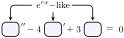
Homogeneous equation diagram: box double-prime minus 4 box prime plus 3 box equals 0, each box filled by e to the r x.
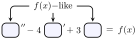
Nonhomogeneous equation diagram: box double-prime minus 4 box prime plus 3 box equals f of x, boxes filled by a form of f.
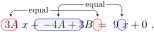
Coefficient-matching: 3 A x plus negative 4 A plus 3 B equals 9 x plus 0; x-terms and constants paired.
Figure 383. Comparison of a homogeneous equation (left) and a nonhomogeneous equation (right). In both, the solutions must simplify in a specific way when substituted into the equation.
Table 384. row 1
\(f(x)\ \) type \(y_p\) Form
1 \(a\) (constant) \(A\)
Table 385. row 2
\(f(x)\ \) type \(y_p\) Form
2 \(ax + b\) \(Ax + B\)
Table 386. row 3
\(f(x)\ \) type \(y_p\) Form
3 \(ax^2 + bx + c\) \(Ax^2 + Bx + C\)
Table 387. row 4
\(f(x)\ \) type \(y_p\) Form
4 \(ax^3 + bx^2 + cx + d\) \(Ax^3 + Bx^2 + Cx + D\)
Table 388. row 5
\(f(x)\ \) type \(y_p\) Form
5 \(a e^{\ds\alpha x}\) \(A e^{\ds\alpha x}\)
Table 389. row 6
\(f(x)\ \) type \(y_p\) Form
6 \(a \sin(\beta x) + b \cos(\beta x)\) \(A \sin(\beta x) + B \cos(\beta x)\)

Worksheet Laplace Transforms

In this section, we introduced the concept of the forward Laplace transform and derived some common Laplace transforms that we will use throughout this chapter. The following points summarize the essential concepts from the forward Laplace transform section:

✳️ Summary of the Key Ideas.

  • Differential \(\to\) Algebraic Equations. The Laplace transform converts a differential equation into an algebraic equation, simplifying the solution process by eliminating derivatives.
  • Laplace Transform Concept. Applying the Laplace transform to a differential equation involves transforming each term by multiplying by \(e^{-st}\) and integrating with respect to \(t\) from \(0\) to \(\infty\text{,}\) but is often simplified by directly applying the Laplace operator, \(\laplacesym\text{.}\)
  • Linearity Property. The Laplace transform is linear, meaning it distributes across addition and subtraction, and allows for constants to be factored out. This property is essential for transforming complex equations.
  • Transforming Initial Conditions. Initial conditions are incorporated directly into the Laplace-transformed equation, modifying the transformed terms to include initial values, making it easier to solve the resulting algebraic equation.
  • Common Function Transforms. The Laplace transforms of common functions, such as exponentials, sines, cosines, and polynomials, are essential tools in transforming differential equations and are summarized in the provided table.
  • Transforming Derivatives. The Laplace transform of a derivative, \(y'(t)\) or higher, transfers the derivative onto the Laplace variable \(s\text{,}\) reducing the order of the equation while introducing initial condition terms.
  • Multiplication by \(e^{at}\) and \(t^n\). When multiplying a function by an exponential \(e^{at}\text{,}\) the Laplace transform shifts by \(a\) in the \(s\)-domain, and multiplying by \(t^n\) corresponds to differentiating the transform \(n\) times with respect to \(s\text{,}\) introducing a sign change.
  • Transforming the Entire Equation. The process of applying the Laplace transform to an entire differential equation with initial conditions involves systematically transforming each term and leads to a simplified algebraic equation in the \(s\)-domain, ready for solving.
Assume \(F(s) = \lap{f(t)}\text{,}\) \(a\text{,}\) \(b\) are constant, and \(n=0,1,2,3,\ldots\)
Table 390. Common Laplace Transforms. \(a, b\) are constant, \(n = 1, 2, \ldots\)
\(t\)-functions \(s\)-functions
\(\downarrow\) \(\downarrow\)
\(f(t)\) \(\lap{ f(t) }\)
\(L_1\) \(1\) \(\ds \frac{1}{s}\) \(s \gt 0\)
\(L_2\) \(e^{at}\) \(\ds \frac{1}{s-a}\) \(s \gt a\)
\(L_3\) \(t^n\) \(\ds \frac{n!}{s^{n+1}}\) \(s \gt 0\)
\(L_4\) \(\sin (bt)\) \(\ds \frac{b}{s^2 + b^2}\) \(s \gt 0\)
\(L_5\) \(\cos(bt)\) \(\ds \frac{s}{s^2 + b^2}\) \(s \gt 0\)
\(L_6\) \(t^n e^{at}\) \(\ds \frac{n!}{(s-a)^{n+1}}\) \(s \gt a\)
\(L_7\) \(e^{at} \sin(bt)\) \(\ds \frac{b}{(s-a)^2 + b^2}\) \(s \gt a\)
\(L_8\) \(e^{at} \cos(bt)\) \(\ds \frac{s-a}{(s-a)^2 + b^2}\) \(s \gt a\)
Table 391. Laplace Transforms Properties, \({\small \lap{ y(t) } = Y(s), \ \lap{ z(t) } = Z(s)}\)
Properties
\(P_1\) \(\ds \lap{ a y(t) \pm b z(t) } = a Y(s) \pm b Z(s) \vphantom{\frac{d}{d}}\)
\(P_2\) \(\ds \lap{ e^{at} y(t) } = Y(s-a) \vphantom{\frac{d}{d}}\)
\(P_3\) \(\ds \lap{ y'(t) } = s\,Y(s) - y(0) \vphantom{\frac{d}{d}}\)
\(P_4\) \(\ds \lap{ y''(t) } = s^2\,Y(s) - s\,y(0) - y'(0) \vphantom{\frac{d}{d}}\)
\(P_5\) \(\ds \lap{ y'''(t) } = s^3\,Y(s) - s^2\,y(0) - s\,y'(0) - y''(0) \vphantom{\frac{d}{d}}\)
\(P_6\) \(\ds \lap{ t^n y(t) } = (-1)^n \frac{d^{(n)}}{ds^{(n)}}Y(s) \vphantom{\frac{d}{d}}\)
Table 392. Table of Common Laplace Transforms
Function
(\(t\)-Domain)
\(f(t)\)
Laplace Transform
(\(s\)-Domain)
\(\lap{f(t)} = F(s)\)

Existence
Condition
L\(_1\) \(1\) \(\ds \frac{1}{s}\) \(s > 0\)
L\(_2\) \(e^{at}\) \(\ds \frac{1}{s - a}\) \(s > a\)
L\(_3\) \(t^n\) \(\ds \frac{n!}{s^{n+1}}\) \(s > 0\)
L\(_4\) \(\sin(bt)\) \(\ds \frac{b}{s^2+b^2}\) \(s > 0\)
L\(_5\) \(\cos(bt)\) \(\ds \frac{s}{s^2+b^2}\) \(s > 0\)
L\(_6\) \(e^{at}\ t^n\) \(\ds \frac{n!}{(s-a)^{n+1}}\) \(s > a\)
L\(_7\) \(e^{at}\sin(bt)\) \(\ds \frac{b}{(s-a)^2+b^2}\) \(s > a\)
L\(_8\) \(e^{at}\cos(bt)\) \(\ds \frac{s-a}{(s-a)^2+b^2}\) \(s > a\)
R\(_{1}\) \(f'(t)\) \(sF(s) - f(0)\) \(s > 0\)
R\(_{2}\) \(f''(t)\) \(s^2F(s) - sf(0) - f'(0)\) \(s > 0\)
R\(_{3}\) \(f'''(t)\) \(s^3F(s) - s^2f(0) - sf'(0) - f''(0)\) \(s > 0\)
R\(_{4}\) \(e^{at} f(t)\) \(F(s-a)\) \(s > 0\)
R\(_{5}\) \(t^n f(t)\) \(\ds (-1)^n \frac{d^n}{ds^n}\Big[F(s)\Big]\) \(s > 0\)
Table 393. L\(_1\)
L\(_1\) \(1\) \(\ds \frac{1}{s}\) \(s > 0\)
Table 394. L\(_2\)
L\(_2\) \(e^{at}\) \(\ds \frac{1}{s - a}\) \(s > a\)
Table 395. L\(_3\)
L\(_3\) \(t^n\) \(\ds \frac{n!}{s^{n+1}}\) \(s > 0\)
Table 396. L\(_4\)
L\(_4\) \(\sin(bt)\) \(\ds \frac{b}{s^2+b^2}\) \(s > 0\)
Table 397. L\(_5\)
L\(_5\) \(\cos(bt)\) \(\ds \frac{s}{s^2+b^2}\) \(s > 0\)
Table 398. L\(_6\)
L\(_6\) \(e^{at}\ t^n\) \(\ds \frac{n!}{(s-a)^{n+1}}\) \(s > a\)
Table 399. L\(_7\)
L\(_7\) \(e^{at}\sin(bt)\) \(\ds \frac{b}{(s-a)^2+b^2}\) \(s > a\)
Table 400. L\(_8\)
L\(_8\) \(e^{at}\cos(bt)\) \(\ds \frac{s-a}{(s-a)^2+b^2}\) \(s > a\)
Table 401. R\(_1\)
Function (\(t\)-Domain) Laplace Transform (\(s\)-Domain) Existence
\(f(t)\) \(\lap{f(t)} = F(s)\) Condition
R\(_{1}\) \(f'(t)\) \(sF(s) - f(0)\) \(s > 0\)
Table 402. R\(_2\)
Function (\(t\)-Domain) Laplace Transform (\(s\)-Domain) Existence
\(f(t)\) \(\lap{f(t)} = F(s)\) Condition
R\(_{2}\) \(f''(t)\) \(s^2F(s) - sf(0) - f'(0)\) \(s > 0\)
Table 403. R\(_3\)
Function (\(t\)-Domain) Laplace Transform (\(s\)-Domain) Existence
\(f(t)\) \(\lap{f(t)} = F(s)\) Condition
R\(_{3}\) \(f'''(t)\) \(s^3F(s) - s^2f(0) - sf'(0) - f''(0)\) \(s > 0\)
Table 404. R\(_4\)
Function (\(t\)-Domain) Laplace Transform (\(s\)-Domain) Existence
\(f(t)\) \(\lap{f(t)} = F(s)\) Condition
R\(_{4}\) \(e^{at} f(t)\) \(F(s-a)\) \(s > 0\)
Table 405. R\(_5\)
Function (\(t\)-Domain) Laplace Transform (\(s\)-Domain) Existence
\(f(t)\) \(\lap{f(t)} = F(s)\) Condition
R\(_{5}\) \(t^n f(t)\) \(\ds (-1)^n \frac{d^n}{ds^n}\Big[F(s)\Big]\) \(s > 0\)

Worksheet Laplace Transform Method

In this section, we introduced the concept of the forward Laplace transform and derived some common Laplace transforms that we will use throughout this chapter. The following points summarize the essential concepts from the forward Laplace transform section:

✳️ Summary of the Key Ideas.

Laplace Transform Method
Common Forms: A table of common Laplace transforms is provided, which doubles as a reference for inverse transforms. The focus is on recognizing forms that match the table entries for functions like \(\sin(bt), \cos(bt)\text{,}\) and others.
Direct Computation: When the function of \(s\) directly matches a form in the common Laplace transform table, the inverse Laplace transform can be easily computed.
Modifying Functions: When a function doesn’t match a known form, minor modifications, such as multiplying by missing constants or splitting fractions, can help.
Completing the Square: When dealing with quadratic expressions in the denominator, especially when the discriminant is negative, completing the square can transform the expression into a form that matches known inverse Laplace transforms. Several examples demonstrate this technique.
Partial Fraction Decomposition: For more complex rational functions, partial fraction decomposition breaks down the function into simpler fractions that match the common transform forms.
Table 406. Matching Guide: \(s\)-function \(\rightarrow\) Inverse Transform
Denominator Form Example Transform
\(\ds \frac{c}{s}\) \(\ds \frac{5}{s}\) L\(_1\)
\(\ds \frac{c}{s^P}\) \(\ds \frac{-10}{s^5}\) L\(_3\)
\(\ds \frac{c}{s\pm a}\) \(\ds \frac{1}{s + 1.8}\) L\(_2\)
\(\ds \frac{c}{(s\pm a)^P}\) \(\ds \frac{6.77}{(s - 3)^9}\) L\(_6\)
\(\ds \frac{cb}{s^2 + b^2}\) \(\ds \frac{\pi}{s^2 + 4}\) L\(_4\)
\(\ds \frac{cs}{s^2 + b^2}\) \(\ds \frac{6s}{s^2 + 3}\) L\(_5\)
\(\ds \frac{cb}{(s \pm a)^2 + b^2}\) \(\ds \frac{1}{(s - 3)^2 + 1}\) L\(_7\)
\(\ds \frac{c(s \pm a)}{(s \pm a)^2 + b^2}\) \(\ds \frac{-0.33(s + 17)}{(s + 17)^2 + 12}\) L\(_8\)

Tips for Preparing the Backward Transform.

Completing the square is an essential technique for transforming quadratic expressions that don’t directly match a form in the table of common Laplace transforms. However, it’s not the only strategy available. In this section, we’ll explore another important technique: partial fraction decomposition. This method is useful for breaking down complex fractions into simpler components that can each be matched with forms in the Laplace transform table.
Two other forms we may wish to match when we study Laplace transforms are
\begin{equation*} \frac{b}{(s-a)^2 + b^2} \mbox{ and } \frac{s-a}{(s-a)^2 + b^2}. \end{equation*}
As before, we work toward making the denominator match first, and then we sort out the numerator second.
When we want to take the inverse Laplace transform of a rational function with a second-degree polynomial in the denominator, we may complete the square or we may do a partial fraction decomposition. How will we know which is appropriate? Here are a few guidelines for you to consider.
  • Does the denominator factor in an obvious way? If so, factor the denominator and do a partial fraction decomposition if necessary.
  • If the denominator does not factor in an obvious way, try completing the square.
  • If you end up with addition outside of the parentheses, as in \((s - a)^2 + b^2,\) then you should aim to match \(L7\) and/or \(L8\).
  • If instead you end up with subtraction outside the parentheses, as in \((s - a)^2 - b^2,\) then you should factor and do a partial fraction decomposition. You may consider using the quadratic formula if the factorization is not obvious to you.
  • If you end up with no terms outside the parentheses, as in \((s - a)^2,\) then use \(L6\).

Worksheet Piecewise Forcing Functions

✳️ Piecewise & Unit Step Functions.

Piecewise Function
A function built from different parts over specific regions of its domain. Each piece has its own behavior, but together they create the entire function.
Unit Step Function
The β€œON-OFF switch” that turns on at \(t = c\text{:}\)
\begin{equation*} u_c(t) = \begin{cases} 0, & t \lt c \\ 1, & t \ge c \end{cases} \end{equation*}
with \(u_0(t) = u(t)\text{.}\)
ON-OFF Switches
Combinations of unit steps turn pieces on over an interval:
\begin{align*} u_c(t) \amp\quad\text{ON for } [c, \infty),\\ u_c(t) - u_d(t) \amp\quad\text{ON for } [c, d),\\ 1 - u_c(t) \amp\quad\text{ON for } (-\infty, c). \end{align*}

✳️ Writing a Piecewise Function with Switches.

Multiply each piece by the switch for its active interval, then add the results. For a three-part function with cut points \(c \lt d\text{:}\)
\begin{align*} P(t) \text{ on } t \lt c \amp\ \longrightarrow\ P(t)\,\big(1 - u_c(t)\big),\\ Q(t) \text{ on } c \le t \lt d \amp\ \longrightarrow\ Q(t)\,\big(u_c(t) - u_d(t)\big),\\ R(t) \text{ on } t \ge d \amp\ \longrightarrow\ R(t)\,u_d(t). \end{align*}

✳️ Transform Rules for Step Functions.

L\(_9\) β€” Transform of a Unit Step
\begin{equation*} \lap{u_c(t)} = \frac{e^{-cs}}{s}, \qquad s \gt 0. \end{equation*}
L\(_{10}\) β€” Forward Transform of \(f(t)\,u_c(t)\)
Used to transform a piecewise term. Replace \(t\) by \(t + c\) inside the function:
\begin{equation*} \lap{f(t)\,u_c(t)} = e^{-cs}\,\lap{f(t + c)}. \end{equation*}
L\(_{11}\) β€” Shifted Function \(f(t - c)\,u_c(t)\)
Best suited to inverse transforms, where you match terms that look like \(e^{-cs}F(s)\text{:}\)
\begin{equation*} \lap{f(t - c)\,u_c(t)} = e^{-cs}F(s), \qquad F(s) = \lap{f(t)}. \end{equation*}
Reading L\(_{11}\) Backward
An exponential factor \(e^{-cs}\) always brings in a switch \(u_c(t)\) and a shift by \(c\text{:}\)
\begin{equation*} \ilap{e^{-cs}F(s)} = f(t - c)\,u_c(t). \end{equation*}

✳️ Laplace Method with Piecewise Forcing.

The big picture is the same three-step Laplace method, with one setup step first.
Setup
Rewrite the forcing term \(g(t)\) in unit step form, combining terms so you have the fewest possible switches.
Step 1 β€” Forward Transform
Transform the equation into the Laplace domain term-by-term, using the derivative rules with the initial conditions and \(L_9\) for the steps.
Step 2 β€” Solve for \(Y(s)\)
Solve algebraically, then prepare each part as \(F(s)\,e^{-cs}\) β€” collect the exponential factors, partial-fraction decompose \(F(s)\text{,}\) and precompute \(f(t) = \ilap{F(s)}\text{.}\)
Step 3 β€” Inverse Transform
Invert each \(F(s)\,e^{-cs}\) with \(L_{11}\) to \(f(t - c)\,u_c(t)\text{,}\) recovering \(y(t)\text{.}\)

Worksheet First-Order Linear Systems

✳️ Systems of Differential Equations.

System of Differential Equations
A collection of differential equations that must be solved together because they track several unknowns that may influence each other. A two-variable first-order system has the form
\begin{align*} \frac{dx}{dt} \amp= a x + b y,\\ \frac{dy}{dt} \amp= c x + d y. \end{align*}
Coupling
A system is uncoupled when neither equation contains the other’s variable, partially coupled when the interaction runs one way, and fully coupled when both variables affect each other so that neither equation stands alone.
Linear System
A system is linear if every equation is linear in its dependent variables β€” the unknowns and their derivatives appear without products, powers, or nonlinear functions. The dimension of the system is the number of dependent variables.

✳️ Matrix Form.

Coefficient Matrix & State Vector
Collecting the constants into the coefficient matrix \(A\) and the unknowns into the state vector \(\vec{X}\) writes the whole system as one compact equation:
\begin{equation*} \frac{d\vec{X}}{dt} = A\vec{X}, \qquad A = \begin{bmatrix} a \amp b \\ c \amp d \end{bmatrix}, \qquad \vec{X} = \begin{bmatrix} x \\ y \end{bmatrix}. \end{equation*}
Second-Order Equation to a System
Any higher-order equation becomes a first-order system by naming the derivatives as new variables. For \(y'' + 3y' + 2y = 0\text{,}\) let \(u = y\) and \(v = y'\text{:}\)
\begin{align*} u' \amp= v,\\ v' \amp= -2u - 3v. \end{align*}

✳️ The Eigenvalue Method.

Eigenvalues & Eigenvectors
Substituting the guess \(\vec{X}(t) = \vec{v}\,e^{rt}\) into \(\vec{X}' = A\vec{X}\) gives the eigenvalue equation
\begin{equation*} A\vec{v} = r\vec{v}. \end{equation*}
The allowed exponential rates \(r\) are the eigenvalues of \(A\text{;}\) the matching vectors \(\vec{v}\) are the eigenvectors.
Characteristic Equation
The eigenvalues are the roots of
\begin{equation*} \det(A - rI) = 0. \end{equation*}
General Solution
For real, distinct eigenvalues \(r_1, r_2\) with eigenvectors \(\vec{v}_1, \vec{v}_2\text{,}\)
\begin{equation*} \vec{X}(t) = C_1 \vec{v}_1 e^{r_1 t} + C_2 \vec{v}_2 e^{r_2 t}. \end{equation*}
For a complex pair \(r = a \pm bi\text{,}\) the real part \(a\) sets a growth factor \(e^{at}\) and the imaginary part \(b\) produces rotation through \(\cos(bt)\) and \(\sin(bt)\text{.}\)

✳️ Qualitative Behavior in the Phase Plane.

A solution traces a trajectory through the phase plane (the \(xy\)-plane); the collection of all trajectories is the phase portrait. For a \(2 \times 2\) system with distinct eigenvalues, the eigenvalues classify the equilibrium at the origin:

Real, both negative \((r_1 < r_2 < 0)\)
Node (sink) β€” every trajectory slides into the origin.
Real, both positive \((0 < r_1 < r_2)\)
Node (source) β€” every trajectory flows away from the origin.
Real, opposite signs \((r_1 < 0 < r_2)\)
Saddle β€” drawn in along one eigenvector, flung out along the other.
Complex \(r = a \pm bi\text{,}\) \(a < 0\)
Spiral sink β€” trajectories loop inward as they decay.
Complex \(r = a \pm bi\text{,}\) \(a > 0\)
Spiral source β€” trajectories loop outward as they grow.
Purely imaginary \(r = \pm bi\)
Center β€” trajectories orbit the origin in closed loops.
In short: the real part of each eigenvalue controls growth or decay, and a nonzero imaginary part adds rotation.
You have attempted of activities on this page.