Section 7.4 Classifying Equilibrium Solutions

Equilibrium solutions mark the places where a system comes to rest. But not all equilibrium solutions are alike; some attract nearby solutions, others repel them, and some do a bit of both. In this section, we’ll learn how to classify these points by examining the slope field, the sign of $f(y)\text{,}$ and a tool called a phase line.

Subsection Types of Equilibria

Suppose $y = c$ is an equilibrium solution of an autonomous equation $y' = f(y)\text{.}$ If you nudge a solution slightly above or below $c\text{,}$ it might drift back, move away, or react differently on each side. What it does determines the type of equilibrium it is.

There are three common types:

Stable (sink): Solutions move toward the equilibrium from both sides.
Unstable (source): Solutions move away from the equilibrium on both sides.
Semi-stable: Solutions move toward the equilibrium on one side and away from it on the other.

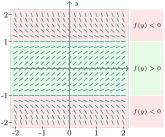
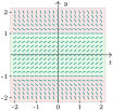
In a slope field, a sink looks like segments converging toward a horizontal line, a source shows segments diverging away, and a semi-stable equilibrium is a mix: converging on one side, diverging on the other. Next, we’ll look at different ways to determine these behaviors.

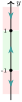
Subsection Classification via the Phase Line

Slope fields convey a great deal of information at once, but for autonomous equations, we can simplify them. Since the slope depends only on $y\text{,}$ we can “compress” the slope field into a simple vertical diagram of just $y$-values. This is called a phase line.

On a phase line:

Equilibria are marked with solid dots.
Regions where $f(y) > 0$ get upward arrows.
Regions where $f(y) < 0$ get downward arrows.

The arrows summarize how $y(t)$ changes: whether solutions are rising or falling. Follow the arrows up or down, and you’ll see where solutions eventually settle—or whether they’re pushed away.

Slope field for y-prime equals 1 minus y squared, shaded green where slopes are positive between y = -1 and 1, red outside. — Figure 98. Slope Field (left) and Phase Line (right) for $y'= 1 - y^2$

Vertical phase line for y-prime equals 1 minus y squared, with arrows showing y = 1 as a sink and y = -1 as a source. — Figure 98. Slope Field (left) and Phase Line (right) for $y'= 1 - y^2$

🌌 Example 99. Growth and Decay.

Find and classify the equilibrium solutions of the autonomous equation:

\begin{equation*} \frac{dy}{dt} = y^2 - 4y \end{equation*}

Solution.

First, set $f(y)=0\text{:}$

\begin{equation*} y^2 - 4y = y(y - 4) = 0, \end{equation*}

giving equilibrium solutions at $y = 0$ and $y = 4\text{.}$

These values split the $y$-axis into three regions. We test the sign of $f(y)$ in each:

Region	Test Point	$f(y) = y(y - 4)$	Sign of $f(y)$
$(-\infty, 0)$	$y = -1$	$(-1)(-5) = 5$	Positive
$(0,4)$	$y = 1$	$(1)(-3) = -3$	Negative
$(4,\infty)$	$y = 5$	$(5)(1) = 5$	Positive

\begin{equation*} \rightarrow \end{equation*}

$Vertical phase line for y-prime equals y squared minus 4y, with equilibria at y = 0, a sink, and y = 4, a source.$

Now we can classify the equilibria based on the phase line:

Solutions move toward $y(t) = 0\text{,}$ so it is a sink.
Solutions move away from $y(t) = 4\text{,}$ so it is a source.

Checkpoint 100. 📖❓ Match the Equilibria.

Suppose an autonomous equation has three equilibrium solutions at

\begin{equation*} y=A,\ y=B,\ \text{and}\ \ y=C\text{.} \end{equation*}

Based on the provided phase line, drag each equilibrium solution to its corresponding classification type.

Phase Line

\begin{equation*} \rightarrow \end{equation*}

$Generic vertical phase line with three equilibria: the top point is a sink, the middle a source, and the bottom semi-stable.$

Three solid dots sit on a vertical line. Arrows point toward the top dot from both sides (a sink), away from the middle dot on both sides (a source), and toward the bottom dot from above but away below (semi-stable). No numeric labels are shown; the points are referred to as A, B, and C in the exercise.

\begin{equation*} \begin{array}{c} A\\ \ds\vphantom{\int} B\\ C \end{array} \end{equation*}

$A$
Sink
$B$
Source
$C$
Semi-stable
None of these

Subsection Classification via the Linearization Method

There’s another way to classify equilibria: use a quick calculus check on $f(y)\text{.}$

Notice in Figure 101 that the sign of $f(y)$ flips as you pass through an equilibrium. The pattern of that flip tells you what kind of point it is:

At the source, $y=-1\text{,}$ $f(y)$ goes from negative → positive (increases).
At the sink, $y=1\text{,}$ $f(y)$ goes from positive → negative (decreases).

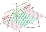
The important observation is that $f(y)$ increases through sources and decreases through sinks. This is true in general, so we can classify equilibrium solutions by looking at the sign of $f'(y)$ at the equilibrium points.

Slope field for y-prime equals 1 minus y squared, shaded by slope sign, converging toward y = 1 and diverging from y = -1. — Figure 101. Slope field for $y' = 1 - y^2\text{.}$

Slope field for y-prime equals 1 minus y squared and the graph of f of y, a downward parabola, linking f’s sign to behavior. — Figure 102. The slope field for $y' = 1 - y^2$ shown alongside the graph of $f(y) = 1 - y^2\text{.}$

If $f(y_0) = 0\text{,}$ then $y_0$ is an equilibrium. To classify it:

If $f'(y_0) < 0\text{,}$ it’s a sink (stable).
If $f'(y_0) > 0\text{,}$ it’s a source (unstable).
If $f'(y_0) = 0\text{,}$ the test is inconclusive—you’ll need more investigation.

This is called the linearization method, because it looks at the linear (slope) behavior of $f(y)$ near the equilibrium.

🌌 Example 103.

Consider the autonomous equation:

\begin{equation*} \frac{dy}{dt} = y^2 - 4y + 3. \end{equation*}

Find and classify the equilibrium solutions using linearization.

Solution.

First, solve $f(y)=0\text{:}$

\begin{equation*} y^2 - 4y + 3 = (y - 1)(y - 3) = 0, \end{equation*}

so $y=1$ and $y=3$ are equilibria.

Then compute the derivative:

\begin{equation*} f'(y) = 2y - 4. \end{equation*}

At each equilibrium:

$f'(1) = -2$ → sink (stable).
$f'(3) = 2$ → source (unstable).

Checkpoint 104. 🤔💭 Classifying Equilibrium Solutions.

(a) 📖❓ Stability Check.

The autonomous equation

\begin{equation*} \frac{dy}{dt} = (y - 3)(y + 1). \end{equation*}

has equilibrium solutions at $y = -1$ and $y = 3\text{.}$ Create a simple phase line to classify these equilibria.

$y = -1$ is a sink, $y = 3$ source
$y = -1$ is a source, $y = 3$ sink
Both are sinks
Both are sources
$y = -1$ is semi-stable, $y = 3$ sink
$y = -1$ is a source, $y = 3$ semi-stable

(b) 📖❓ Comparing Equilibria.

The equation

\begin{equation*} \frac{dy}{dt} = y^2-3y \end{equation*}

has equilibrium solutions at $y=0$ and $y=3\text{.}$

Compute $f'(y)$ and use the linearization method to determine which of these equilibria pulls nearby solutions toward it.

$y=0$
Correct. Since $f'(y) = 2y-3$ and $f'(0) = -3 \lt 0\text{,}$ then $y=0$ is a sink and pulls solutions toward it.
$y=3$
Incorrect. Since $f'(y) = 2y-3$ and $f'(3) = +3 \gt 0\text{,}$ then $y=3$ is a source and repels solutions.

You have attempted of activities on this page.

Prev Top Next

Region	Test Point	\(f(y) = y(y - 4)\)	Sign of \(f(y)\)
\((-\infty, 0)\)	\(y = -1\)	\((-1)(-5) = 5\)	Positive
\((0,4)\)	\(y = 1\)	\((1)(-3) = -3\)	Negative
\((4,\infty)\)	\(y = 5\)	\((5)(1) = 5\)	Positive