When working with first-order differential equations, you can gain insight into solutions without fully solving them. By focusing on how the solutions change, you can use a slope field to visualize the path of any potential solution.
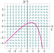
A slope field visually represents the slopes that a solution curve must follow at each point in the plane, shown as short segments tracing the way a solution would travel—like a leaf carried by a stream.
The pattern created by a slope field provides a visual representation of the family of solutions to the differential equation. A slope field doesn’t show just one solution—it shows them all. From any starting point, a solution curve threads through, always guided by the tiny segments.
How many curves thread through each point? Under the mild smoothness conditions of the existence and uniqueness result from the solutions chapter, exactly one — which is why the solution curves in a slope field never cross each other. Where those conditions fail, curves really can merge or split (as in 🌌 Example 38), so the never-crossing rule is a theorem, not a coincidence.
Here \(f(t,y)\) is the “slope generator”: given any point \((t,y)\text{,}\) it outputs the slope the solution must have there. For instance, if \(t=3\) and \(y=5\text{,}\)
Sketching by hand is great for intuition, but tedious when you need more points. Computer-generated slope fields fill in the gaps, revealing a dense web of segments that paints the full picture. In Figure 91, the solution curve through \((0,\frac12)\) flows smoothly along the segments, like an object carried by a current.
A slope field turns an equation into a navigational chart. Each segment is an instruction every solution must obey. The entire field represents the whole family of solutions, letting you spot patterns in how solutions behave, without ever solving for \(y\) explicitly. Next, we’ll look at autonomous equations, whose slope fields reveal even more structure.