Section 15.2 Nullclines and the Phase Plane

Knowing where the equilibria sit is only half a picture. We also want to know what the flow does between them: which way trajectories travel, whether they circle, and which equilibrium they head toward.

Drawing a full direction field by hand means evaluating \((f,g)\) at dozens of points. Nullclines give us the same information for a fraction of the work. They are the phase-plane cousin of the phase line from Qualitative Methods: a few curves that carve the plane into regions, with the direction of motion constant in sign throughout each region.

Subsection Curves Where One Variable Stops

An equilibrium needs both derivatives to vanish. A nullcline asks for only one at a time.

📙 Definition 321. Nullclines.

For the system \(x' = f(x,y)\text{,}\) \(y' = g(x,y)\text{:}\)

The x-nullclines are the curves where \(f(x,y) = 0\text{.}\) Crossing one, \(x\) is momentarily not changing, so the motion there is purely vertical.
The y-nullclines are the curves where \(g(x,y) = 0\text{.}\) There \(y\) is momentarily not changing, so the motion is purely horizontal.

Two consequences follow immediately, and they are what make nullclines worth drawing.

Equilibria are the crossings. A point where an \(x\)-nullcline meets a \(y\)-nullcline has \(f = 0\) and \(g = 0\) — the definition of an equilibrium point. Two \(x\)-nullclines crossing each other is not enough; the curves must come from different equations.
Signs are constant in between. Because \(f\) can only change sign by passing through zero, the sign of \(x'\) is the same everywhere inside a region bounded by \(x\)-nullclines. The same is true of \(y'\text{.}\) So a single test point per region determines the direction of the flow across the entire region.

The result is a coarse map of the phase plane: four possible arrow directions (up-right, up-left, down-left, down-right), one per region, sketched from a handful of arithmetic checks.

Subsection Mapping the Flow: A Worked Example

We return to the rabbits and foxes of 🌌 Example 318:

\begin{align*} \frac{dR}{dt} \amp = R(0.5 - 0.02F)\\ \frac{dF}{dt} \amp = F(-0.3 + 0.01R) \end{align*}

Only the biologically meaningful quadrant \(R \geq 0\text{,}\) \(F \geq 0\) concerns us.

🌌 Example 322. Nullclines of the Predator-Prey Model.

Find the nullclines of the rabbit-fox system and use them to determine the direction of motion in each region of the first quadrant.

Solution.

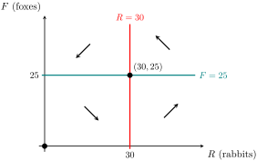
Step 1: the nullclines. Setting \(dR/dt = 0\) gives \(R = 0\) (the vertical axis) or \(F = 25\) (a horizontal line). Setting \(dF/dt = 0\) gives \(F = 0\) (the horizontal axis) or \(R = 30\) (a vertical line).

The two axes are nullclines as well as boundaries, which matches the biology: with no rabbits, or no foxes, one population is stuck at zero forever. Inside the quadrant, the interesting curves are the line \(F = 25\) (where \(R\) pauses) and the line \(R = 30\) (where \(F\) pauses). They cross at \((30,25)\) — the coexistence equilibrium.

Step 2: sign of each derivative. Read the factored form directly:

\begin{align*} R' \amp \gt 0 \text{ when } F \lt 25, \amp\quad R' \amp \lt 0 \text{ when } F \gt 25,\\ F' \amp \gt 0 \text{ when } R \gt 30, \amp\quad F' \amp \lt 0 \text{ when } R \lt 30 . \end{align*}

(Both statements assume \(R \gt 0\) and \(F \gt 0\text{,}\) so the leading factors are positive.)

Step 3: assemble the four regions.

Region	Sign of \(R'\)	Sign of \(F'\)	Motion
\(R \lt 30\text{,}\) \(F \lt 25\)	+	\(-\)	right and down
\(R \gt 30\text{,}\) \(F \lt 25\)	+	+	right and up
\(R \gt 30\text{,}\) \(F \gt 25\)	\(-\)	+	left and up
\(R \lt 30\text{,}\) \(F \gt 25\)	\(-\)	\(-\)	left and down

Follow those four rows around the table and the arrows chase each other counterclockwise about \((30,25)\text{.}\) That is the predator-prey cycle in its rawest form: plentiful rabbits feed a fox boom, the fox boom eats the rabbits down, the starving foxes decline, and the rabbits recover to start again.

Rabbit-fox phase plane with nullclines at F = 25 and R = 30 crossing at the equilibrium (30, 25), arrows in all four regions. — Figure 323. Nullclines of the rabbit-fox system in the first quadrant. The line \(F = 25\) (where \(R' = 0\)) and the line \(R = 30\) (where \(F' = 0\)) cross at the coexistence equilibrium \((30,25)\) and split the quadrant into four regions. The arrow in each region shows the direction of motion there; together they circulate counterclockwise.

Two cautions about what this picture does and does not say. First, nullclines give directions, not speeds: an arrow says “up and to the right,” not how steeply. Second — and this is the important one — a counterclockwise circulation is consistent with closed loops, with an inward spiral, and with an outward spiral. Nullclines cannot tell those three apart. Settling that question is what Linearization and the Jacobian is for.

Subsection Nullclines That Are Not Straight Lines

Nothing in the definition requires a nullcline to be a line. For the competing species of 🌌 Example 319,

\begin{align*} \frac{dx}{dt} \amp = x(3 - x - 2y)\\ \frac{dy}{dt} \amp = y(2 - x - y) \end{align*}

the \(x\)-nullclines are \(x = 0\) and the line \(x + 2y = 3\text{;}\) the \(y\)-nullclines are \(y = 0\) and the line \(x + y = 2\text{.}\) Four curves, and their crossings are precisely the four equilibria we already found — a useful check on the algebra.

Change the model slightly, to \(x' = x(3 - x^2 - 2y)\text{,}\) and the \(x\)-nullcline becomes the parabola \(y = (3-x^2)/2\text{.}\) The method does not change at all: draw the curves, pick one test point per region, record the two signs.

✳️ The Nullcline Recipe.

Set \(f(x,y) = 0\) and sketch every resulting curve. These are the \(x\)-nullclines: motion across them is vertical.
Set \(g(x,y) = 0\) and sketch every resulting curve. These are the \(y\)-nullclines: motion across them is horizontal.
Mark each crossing of an \(x\)-nullcline with a \(y\)-nullcline. Those are the equilibria.
In each region, test one convenient point to get the signs of \(f\) and \(g\text{,}\) and draw the corresponding arrow.

Checkpoint 324. 🤔💭 Nullclines Reading Questions.

(a) 📖❓ What Happens on an x-Nullcline?

A trajectory crosses an \(x\)-nullcline. At the moment of crossing, its motion is

purely vertical.
Correct — \(x' = 0\) there, so only \(y\) is changing.
purely horizontal.
That describes a \(y\)-nullcline, where \(y' = 0\text{.}\)
zero — the trajectory stops.
Only if it is also on a \(y\)-nullcline. One vanishing derivative is not an equilibrium.
at \(45^\circ\) to the axes.
Nothing forces a particular angle; what is forced is that the horizontal component is zero.

(b) 📖❓ Where Are the Equilibria?

Which crossings in a nullcline sketch are equilibrium points?

Crossings of an \(x\)-nullcline with a \(y\)-nullcline.
Correct — those are the points where \(f\) and \(g\) both vanish.
Every crossing of any two nullclines.
Two \(x\)-nullclines crossing gives \(f = 0\) twice over, and says nothing about \(g\text{.}\)
Only crossings that lie on an axis.
The coexistence equilibrium \((30,25)\) is a crossing well inside the quadrant.
Only crossings at the origin.
That would be true of most linear systems, not of nonlinear ones.

(c) 📖❓ Find the Nullclines.

For \(x' = x(4 - y)\text{,}\) \(y' = y(x - 3)\text{,}\) select every nullcline listed below.

\(x = 0\) (an \(x\)-nullcline)
\(y = 4\) (an \(x\)-nullcline)
\(x = 3\) (a \(y\)-nullcline)
\(y = 3\) (a \(y\)-nullcline)
Setting \(y' = y(x-3) = 0\) gives \(y = 0\) or \(x = 3\text{,}\) not \(y = 3\text{.}\)
\(x = 4\) (an \(x\)-nullcline)
Setting \(x' = x(4-y) = 0\) gives \(x = 0\) or \(y = 4\text{.}\)

(d) 📖❓ Reading a Region.

In one region of a phase plane a test point gives \(f \lt 0\) and \(g \gt 0\text{.}\) Trajectories in that region move

up and to the left.
Correct: \(x' \lt 0\) means leftward, \(y' \gt 0\) means upward.
up and to the right.
Rightward motion needs \(f \gt 0\text{.}\)
down and to the left.
Downward motion needs \(g \lt 0\text{.}\)
It cannot be determined without solving the system.
The two signs are exactly what determines the direction — no solving required.

(e) 📖❓ How Much Do Nullclines Settle?

A nullcline sketch shows the flow circulating counterclockwise around an equilibrium. What can you conclude?

Nearby trajectories rotate around it, but they could spiral in, spiral out, or close into loops.
Correct — nullclines give direction only. Distinguishing the three cases requires linearization.
The equilibrium is stable.
An outward spiral also circulates. Circulation alone says nothing about stability.
The trajectories are exact closed loops.
Closed loops are only one of the three possibilities consistent with the picture.
The system must be linear.
Circulation happens in both linear and nonlinear systems.

You have attempted of activities on this page.

Prev Top Next