Section 7.3 Equilibrium Solutions

Autonomous equations indicate that the direction of change depends only on the current state, not on the current time. That pattern shows up in their slope fields as horizontal โ€œstripesโ€ of identical slope behavior. We now focus on one particularly important feature of those fields: the horizontal lines where the slope is zero. Along those lines, the system simply stops changing. These constant solutions are called equilibrium solutions.

Subsection Flat Lines and Fixed Behavior

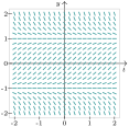
Consider the slope field for the autonomous equation:
\begin{equation*} \frac{dy}{dt} = 1 - y^2\text{.} \end{equation*}
Since this is autonomous, the slope depends only on \(y\text{.}\) At certain \(y\)-values, something special happens: the slope becomes exactly zero.
Slope field for y-prime equals 1 minus y squared, with horizontal, zero-slope segments along y = -1 and y = 1.
Figure 95. Slope field for \(y' = 1 - y^2\)
In the slope field, those points appear as rows of perfectly horizontal segments. Thatโ€™s no accident โ€” where \(dy/dt = 0\text{,}\) the solution curve doesnโ€™t move. If a solution starts there, it stays there forever. These flat lines are the equilibrium solutions.
To find them, we set \(\frac{dy}{dt}\) (the slope) to zero and solve for \(y\text{.}\) In this example:
\begin{equation*} \us{\large =\ 0}{\boxed{\frac{dy}{dt}}} = 1 - y^2 \quad\rightarrow\quad 0 = 1 - y^2 \quad\Rightarrow\quad y = -1 \text{ or } y = 1. \end{equation*}
So the equilibrium solutions are the constant functions \(y(t) = -1\) and \(y(t) = 1\text{.}\)
These constant solutions act like anchors in the system: other solutions either drift toward them or get pushed away. Weโ€™ll explore that stability behavior in the next section.

Checkpoint 96. ๐Ÿ“–โ“ Observing the Slope Field.

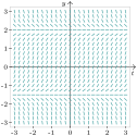
Look at the slope field below. Which constant solutions do you see? In other words, what \(y\)-values have perfectly horizontal segments?
Slope field of an autonomous equation with horizontal, zero-slope segments marking equilibria along y = -1.5 and y = 2.
  • \(y(t) = -2\)
  • \(y(t) = -1.5\)
  • \(y(t) = 0\)
  • \(y(t) = 1.5\)
  • \(y(t) = 2\)

Subsection What the Slope Field Tells You

What about the other values of \(y\text{?}\) Between the equilibria at \(y = -1\) and \(y = 1\text{,}\) the slopes are positive. For example:
\begin{equation*} f(-0.5) = 1 - (-0.5)^2 = 0.75, \end{equation*}
so the slope is positive and solutions rise. The slope field shows this: between \(y=-1\) and \(y=1\text{,}\) the little segments tilt upward.
Above \(y = 1\text{,}\) things flip. Try \(y = 1.5\text{:}\)
\begin{equation*} f(1.5) = 1 - (1.5)^2 = -1.25, \end{equation*}
which is negative, so solutions decrease. The slope field confirms it โ€” segments tilt downward. The same downward pull appears below \(y = -1\text{.}\)
The slope field acts like a behavior map: equilibrium solutions mark where the system is still, while the tilts around them reveal which way nearby solutions move.

Subsection How to Find Equilibrium Solutions

Finding equilibrium solutions is always the same quick process:
  1. Assuming \(c\) is constant and \(y=c\text{,}\) then \(\frac{dy}{dt} = 0\) and so:
    \begin{equation*} \frac{dy}{dt} = f(y) \quad\rightarrow\quad 0 = f(c)\text{.} \end{equation*}
  2. The equation \(f(c) = 0\) is algebraic. Solve it for \(c\text{.}\)
  3. For each \(c\) you found, \(y(t) = c\) is an equilibrium solution.
Letโ€™s do a quick example. Consider:
\begin{equation*} \frac{dy}{dt} = y^2 - 4y. \end{equation*}
Assuming \(y=c\text{,}\) then this equation becomes:
\begin{equation*} 0 = c^2 - 4c \quad\Rightarrow\quad c(c - 4) = 0. \end{equation*}
So, \(c=0, 4\) and the equilibrium solutions are:
\begin{equation*} y(t) = 0 \quad \text{and} \quad y(t) = 4. \end{equation*}
Mark these on the slope field with horizontal lines. Then check the arrows just above and below each line to see how other solutions evolve โ€” whether theyโ€™re pulled in or pushed away. We will build more on this in the next section.
Checkpoint 97. ๐Ÿ“–โ“ Select the Equilibrium Solutions.

Determine the equilibrium solutions for the equation:
\begin{equation*} \frac{dy}{dt} = y + \frac12y^2\text{.} \end{equation*}
Select all that apply.
  • \(\ y(t) = 0\)
  • Yes! โœ…
  • \(\ y(t) = 2\)
  • โŒ
  • \(\ y(t) = -2\)
  • Yes! โœ…
  • \(\ y(t) = -\sqrt{2}\)
  • โŒ
  • \(\ y(t) = -\sfrac12\)
  • โŒ
You have attempted of activities on this page.