Consider the function \(f(x,y) = 1 + x^2 + y^2\text{,}\) the point \(P_0(1,1)\text{,}\) and the unit vector \(\mathbf u = \frac{1}{\sqrt 2}\,\mathbf i +
\frac{1}{\sqrt 2}\,\mathbf j\text{.}\) Estimate the change in the value of \(f\) as a result of moving away from \(P_0(1,1)\) in the direction of \(\mathbf u\) by \(0.1\) units.
Section 8.3 Estimating the Change in a Particular Direction
Consider the function \(z = f(x,y)\text{,}\) a point \(P_0(x_0,y_0)\) in its domain, and a unit vector \(\mathbf u = u_1\,\mathbf i + u_2\,\mathbf j\text{.}\) The question is:
How can we estimate the change in \(f\) (\(\Delta f\)) as a result of moving a small distance (\(ds\)) away from \(P_0\) in the direction \(\mathbf u\text{?}\)
Moving away from \(P_0(x_0,y_0)\) by the distance \(ds\) in the direction \(\mathbf u\) is the displacement \(\mathbf u\,ds = u_1\,ds\,\mathbf i + u_2\,ds\,\mathbf j\text{,}\) with \(|\mathbf u\,ds| = ds\text{,}\) and it takes us to the point \(P(x_0 + u_1\,ds,\; y_0 + u_2\,ds)\text{.}\) As Figure 8.5 shows, this causes the change
\begin{equation}
\Delta f = f(x_0 + u_1\,ds,\; y_0 + u_2\,ds) - f(x_0, y_0)\tag{8.14}
\end{equation}
in the value of the function.
Diagram Exploration Keyboard Controls
We know from (7.5) that the rate of change of \(f\) at a point \(P_0\) in the direction of \(\mathbf u\) is given by the directional derivative
\begin{equation}
\left(\frac{df}{ds}\right)_{\mathbf u, P_0}
= \nabla f \Big|_{P_0} \cdot \mathbf u.\tag{8.15}
\end{equation}
Hence, we can estimate the change in \(f\) as
\begin{equation}
\Delta f \approx df
= \left(\nabla f \Big|_{P_0} \cdot \mathbf u\right) ds.\tag{8.16}
\end{equation}
The quantity \(df\) is called the differential of \(f\text{.}\)
Example 8.6. Estimating the Change in a Given Direction.
Solution.
Note that from the question we know \(ds = 0.1\) units. Our goal is to estimate the change in \(f\text{.}\) We compute the gradient of \(f\) and evaluate it at \(P_0\text{:}\)
\begin{align*}
\nabla f \amp= 2x\,\mathbf i + 2y\,\mathbf j\\
\nabla f \Big|_{(1,1)} \amp= 2\,\mathbf i + 2\,\mathbf j.
\end{align*}
By (8.16),
\begin{align}
df \amp= \left(\nabla f \Big|_{P_0} \cdot \mathbf u\right) ds\notag\\
\amp= \left(\langle 2, 2 \rangle \cdot
\Bigl\langle \frac{1}{\sqrt 2}, \frac{1}{\sqrt 2} \Bigr\rangle\right)(0.1)\notag\\
\amp= 0.2\sqrt 2 \approx 0.28 \text{ units}.\tag{8.17}
\end{align}
For comparison, the exact change is
\begin{align*}
\Delta f \amp= f\left(1 + \frac{0.1}{\sqrt 2},\,
1 + \frac{0.1}{\sqrt 2}\right) - f(1,1)\\
\amp= \left(3 + 0.2\sqrt 2 + 0.01\right) - 3
= 0.2\sqrt 2 + 0.01,
\end{align*}
so the estimate \(df\) is off by only \(0.01\) units. The right panel of Figure 8.7 zooms in on the stretch just past \(P_0\) and shows this gap between the tangent line and the surface.
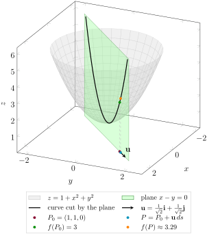
An upward-opening gray paraboloid, the graph of z equals 1 plus x squared plus y squared, cut by a green vertical plane through the line y equals x. The plane meets the surface along a black parabola, and the branch of that parabola through the point 1, 1 faces the viewer. On the base plane, a black arrow shows the unit vector u leaving the point 1, 1, 0. Four points are marked: the input point 1, 1, 0 in dark red, the moved input point in light blue just beyond it, the output point 1, 1, 3 in green on the curve, and the moved output point in orange on the curve; a dashed gray segment joins each input point to its output point. A legend below the picture names the surface, the plane, the curve, the vector u, and the four points.
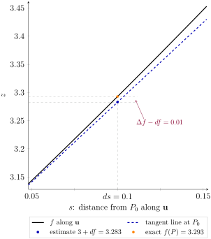
A two dimensional graph zoomed into the neighborhood of the moved point. The horizontal axis is the distance s travelled from P 0 in the direction of u, running from 0.05 to 0.15 rather than from 0, so that the two graphs are far enough apart to be told apart; the vertical axis is z, running from about 3.13 to about 3.46. A black curve is the value of f along u, and a blue dashed line is its tangent line at P 0. The line stays just below the curve and the gap between them widens to the right. At s equals d s equals 0.1, dashed guide lines pick out the two heights: the tangent line reaches the blue point at 3.283, the estimate 3 plus d f, and the curve reaches the orange point at 3.293, the exact value of f at the moved point. A callout labels the gap between the two points as delta f minus d f equals 0.01. A legend below the picture names the curve, the tangent line, and the two marked values.
You have attempted of activities on this page.

