
Section 7.5 Directions of Fastest Increase, Fastest Decrease, and No Change

The directional derivative can be expressed as
\begin{align} D_{\mathbf u} f \amp= \nabla f\cdot\mathbf u\notag\\ \amp= |\nabla f|\,|\mathbf u|\cos\theta\notag\\ \amp= |\nabla f|\cos\theta,\tag{7.11} \end{align}
where \(\theta\) is the angle between \(\nabla f\) and the unit vector \(\mathbf u\text{.}\) This formula has three important consequences:
  • When \(\nabla f\) and \(\mathbf u\) are in the same direction (\(\cos\theta = 1\)), \(f\) increases most rapidly and \(D_{\mathbf u} f = |\nabla f|\text{.}\)
  • When \(\nabla f\) and \(\mathbf u\) have opposite directions (\(\cos\theta = -1\)), \(f\) decreases most rapidly and \(D_{\mathbf u} f = -|\nabla f|\text{.}\)
  • When \(\nabla f\) and \(\mathbf u\) are orthogonal (\(\cos\theta = 0\)), \(f\) does not change, and \(D_{\mathbf u} f = 0\text{.}\)
Diagram Exploration Keyboard Controls
Key Action
Enter, A Activate keyboard driven exploration
B Activate menu driven exploration
Escape Leave exploration mode
Cursor down Explore next lower level
Cursor up Explore next upper level
Cursor right Explore next element on level
Cursor left Explore previous element on level
X Toggle expert mode
W Extra details if available
Space Repeat speech
M Activate step magnification
Comma Activate direct magnification
N Deactivate magnification
Z Toggle subtitles
C Cycle contrast settings
T Monochrome colours
L Toggle language (if available)
K Kill current sound
Y Stop sound output
O Start and stop sonification
P Repeat sonification output
Figure 7.16. Directions around \(P_0\text{:}\) \(f\) increases fastest along \(\nabla f\text{,}\) decreases fastest along \(-\nabla f\text{,}\) and does not change in the two directions orthogonal to \(\nabla f\text{.}\)

Activity 7.5.1. Verifying the Three Special Directions.

The three cases listed above are all consequences of a single formula, \(D_{\mathbf u} f = |\nabla f|\cos\theta\text{.}\) In this activity you will derive them yourself and then check your answers against FigureΒ 7.17, where \(\mathbf u\) can be dragged around the circle of directions.

(a)

Beginning with \(D_{\mathbf u} f = \nabla f \cdot \mathbf u\text{,}\) explain why the dot product can be rewritten as \(|\nabla f|\cos\theta\text{.}\) Where is the assumption \(|\mathbf u| = 1\) used?
Answer.
For any two vectors, \(\mathbf a \cdot \mathbf b = |\mathbf a||\mathbf b|\cos\theta\) with \(\theta\) the angle between them. Applying this to \(\nabla f\) and \(\mathbf u\text{,}\)
\begin{align*} D_{\mathbf u} f = \nabla f \cdot \mathbf u\\ \amp= |\nabla f|\,|\mathbf u|\cos\theta\\ \amp= |\nabla f|\cos\theta , \end{align*}
where the last step uses \(|\mathbf u| = 1\text{.}\) Without that assumption the factor \(|\mathbf u|\) would survive, and rescaling \(\mathbf u\) would change \(D_{\mathbf u} f\) without changing the direction being measured.

(b)

Treat \(|\nabla f|\) as fixed and let \(\theta\) run over \([0, 2\pi)\text{.}\) What are the largest and smallest values of \(D_{\mathbf u} f\text{,}\) and at which angles do they occur? For which angles is \(D_{\mathbf u} f = 0\text{?}\)
Answer.
Since \(-1 \le \cos\theta \le 1\text{,}\) the quantity \(|\nabla f|\cos\theta\) ranges between \(-|\nabla f|\) and \(|\nabla f|\text{.}\) The largest value \(|\nabla f|\) occurs at \(\theta = 0\text{,}\) with \(\mathbf u\) pointing along \(\nabla f\text{;}\) the smallest, \(-|\nabla f|\text{,}\) occurs at \(\theta = \pi\text{,}\) with \(\mathbf u\) pointing along \(-\nabla f\text{.}\) The directional derivative vanishes when \(\cos\theta = 0\text{,}\) that is at \(\theta = \pi/2\) and \(\theta = 3\pi/2\text{,}\) the two directions orthogonal to \(\nabla f\text{.}\)

(c)

Now take \(f(x,y) = 1 + x^2 + y^2\) at \(P_0(1,1)\text{,}\) the function of ExampleΒ 7.6. Compute \(\nabla f\) and \(|\nabla f|\) at \(P_0\text{,}\) write \(D_{\mathbf u} f\) as a function of \(\theta\text{,}\) and give the three special unit vectors explicitly.
Answer.
Here \(\nabla f = 2x\,\mathbf i + 2y\,\mathbf j\text{,}\) so \((\nabla f)_{(1,1)} = 2\,\mathbf i + 2\,\mathbf j\) and \(|\nabla f| = 2\sqrt 2\text{.}\) Therefore
\begin{gather*} D_{\mathbf u} f = 2\sqrt 2 \,\cos\theta . \end{gather*}
The fastest increase happens along \(\mathbf u = \frac{1}{\sqrt 2}\mathbf i + \frac{1}{\sqrt 2}\mathbf j\text{,}\) giving \(D_{\mathbf u} f = 2\sqrt 2 \approx 2.83\text{,}\) which is the value computed in ExampleΒ 7.6. The fastest decrease happens along \(-\frac{1}{\sqrt 2}\mathbf i - \frac{1}{\sqrt 2}\mathbf j\text{,}\) giving \(-2\sqrt 2\text{.}\) There is no change along \(\pm\left(\frac{1}{\sqrt 2}\mathbf i - \frac{1}{\sqrt 2}\mathbf j\right)\text{,}\) the two directions orthogonal to \(\nabla f\text{.}\)

(d)

Check your work against the figure below. Drag \(\mathbf u\) around the circle and confirm that the meter agrees with \(2\sqrt 2\cos\theta\) at several angles. Then use the three buttons and compare the readings with your answers to the previous task. As you drag, at what angle does the reading change most quickly, and at what angle is it momentarily stationary?
Instructions.
Drag the blue unit vector \(\mathbf u\) around the circle of directions and watch the meter display \(D_{\mathbf u} f = |\nabla f|\cos\theta\text{.}\) Use the buttons to snap \(\mathbf u\) to the three special cases: the same direction as \(\nabla f\) (fastest increase), the opposite direction (fastest decrease), and a direction orthogonal to \(\nabla f\) (no change).
Figure 7.17. The directional derivative \(D_{\mathbf u} f = |\nabla f|\cos\theta\) as the unit vector \(\mathbf u\) rotates around \(P_0\text{.}\)
Answer.
The three buttons should give \(2\sqrt 2 \approx 2.83\text{,}\) \(-2\sqrt 2 \approx -2.83\text{,}\) and \(0\text{.}\) The reading changes fastest where \(\left|\frac{d}{d\theta}\cos\theta\right| = |\sin\theta|\) is largest, namely at \(\theta = \pi/2\) and \(3\pi/2\text{,}\) the very directions where \(D_{\mathbf u} f\) itself is zero. It is momentarily stationary at \(\theta = 0\) and \(\theta = \pi\text{,}\) where \(D_{\mathbf u} f\) is largest and smallest. So a small change of heading matters least when you are already pointing straight uphill, and most when you are moving along a level direction.

Example 7.18. Example III.

Consider the function \(f(x,y) = \dfrac{x^2}{2} + \dfrac{y^2}{2}\text{.}\) Find the directions in which, at the point \(P_0(1,1)\text{,}\)
  1. \(f\) increases most rapidly,
  2. \(f\) decreases most rapidly,
  3. there is no change in \(f\text{.}\)
Solution.
A. As explained above, \(f\) increases most rapidly in the direction of \(\nabla f\text{.}\) We have
\begin{align} \nabla f \amp= x\,\mathbf i + y\,\mathbf j \quad\Rightarrow\quad \left(\nabla f\right)_{(1,1)}\notag\\ \amp= \mathbf i + \mathbf j.\tag{7.12} \end{align}
Note that we need to divide \(\left(\nabla f\right)_{(1,1)} = \mathbf i + \mathbf j\) by its length to find the unit vector corresponding to the direction of most rapid increase:
\begin{equation} \frac{\left(\nabla f\right)_{(1,1)}}{\left|\left(\nabla f\right)_{(1,1)}\right|} = \frac{1}{\sqrt 2}\mathbf i + \frac{1}{\sqrt 2}\mathbf j.\tag{7.13} \end{equation}
B. For the direction of most rapid decrease, we take the opposite direction:
\begin{equation} -\frac{\left(\nabla f\right)_{(1,1)}}{\left|\left(\nabla f\right)_{(1,1)}\right|} = -\frac{1}{\sqrt 2}\mathbf i - \frac{1}{\sqrt 2}\mathbf j.\tag{7.14} \end{equation}
C. To find the directions of zero change in \(f\text{,}\) we require
\begin{align} \left(\nabla f\right)_{(1,1)}\cdot\mathbf u \amp= (\mathbf i + \mathbf j)\cdot(u_1\mathbf i + u_2\mathbf j)\notag\\ \amp= u_1 + u_2\notag\\ \amp= 0 \quad\text{or}\quad u_1\notag\\ \amp= -u_2,\tag{7.15} \end{align}
and since \(\mathbf u\) is a unit vector, we have
\begin{equation} |\mathbf u|^2 = u_1^2 + u_2^2 = 1.\tag{7.16} \end{equation}
After substituting (7.15) in (7.16), we conclude
\begin{equation} 2u_1^2 = 1 \quad\Rightarrow\quad u_1 = \pm\frac{1}{\sqrt 2}.\tag{7.17} \end{equation}
Hence, the directions of zero change in \(f\) at \(P_0(1,1)\) are
\begin{align} \mathbf u \amp= \frac{1}{\sqrt 2}\mathbf i - \frac{1}{\sqrt 2}\mathbf j \qquad\text{and}\qquad \tilde{\mathbf u}\notag\\ \amp= -\frac{1}{\sqrt 2}\mathbf i + \frac{1}{\sqrt 2}\mathbf j.\tag{7.18} \end{align}
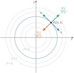
Note that \(\tilde{\mathbf u} = -\mathbf u\text{.}\) All four directions are shown in FigureΒ 7.19 and FigureΒ 7.20: the directions of zero change are tangent to the level curve of \(f\) through \(P_0(1,1)\text{,}\) while the directions of most rapid increase and decrease are perpendicular to it.
Circular level curves with the four special directions marked at the point one comma one.
Concentric circles, the level curves of \(f(x,y) = x^2/2 + y^2/2\text{,}\) centered at the origin. At the point \(P_0(1,1)\text{,}\) four unit arrows are drawn: a green arrow pointing outward along the gradient (fastest increase), a vermillion arrow pointing inward opposite to the gradient (fastest decrease), and two dashed blue arrows tangent to the level circle through \(P_0\) (zero change). A dashed tangent line to the circle at \(P_0\) contains the two blue arrows.
Figure 7.19. The level curves of \(f(x,y) = \frac{x^2}{2} + \frac{y^2}{2}\) are circles centered at the origin. At \(P_0(1,1)\text{,}\) the direction of fastest increase points along \(\nabla f\text{,}\) the direction of fastest decrease points along \(-\nabla f\text{,}\) and the two directions of zero change are tangent to the level curve through \(P_0\text{.}\)
Diagram Exploration Keyboard Controls
Key Action
Enter, A Activate keyboard driven exploration
B Activate menu driven exploration
Escape Leave exploration mode
Cursor down Explore next lower level
Cursor up Explore next upper level
Cursor right Explore next element on level
Cursor left Explore previous element on level
X Toggle expert mode
W Extra details if available
Space Repeat speech
M Activate step magnification
Comma Activate direct magnification
N Deactivate magnification
Z Toggle subtitles
C Cycle contrast settings
T Monochrome colours
L Toggle language (if available)
K Kill current sound
Y Stop sound output
O Start and stop sonification
P Repeat sonification output
Figure 7.20. At \(P_0(1,1)\text{:}\) fastest increase along \(\nabla f/|\nabla f|\text{,}\) fastest decrease along \(-\nabla f/|\nabla f|\text{,}\) and zero change along \(\pm\mathbf u\text{,}\) tangent to the level curve \(f = 1\text{.}\)
Instructions.
Drag the unit vector \(\mathbf u\) around the point \(P_0(1,1)\) on the level-curve plot of \(f(x,y) = \frac{x^2}{2} + \frac{y^2}{2}\) and watch the value of \(D_{\mathbf u} f = u_1 + u_2\text{.}\) Use the buttons to snap \(\mathbf u\) to the answers of Example III: the direction of fastest increase, the direction of fastest decrease, and the two directions of no change.
Figure 7.21. The value of \(D_{\mathbf u} f = u_1 + u_2\) for \(f(x,y)=\frac{x^2}{2}+\frac{y^2}{2}\) as \(\mathbf u\) rotates around \(P_0(1,1)\text{,}\) with the special directions of Example III.
Instructions.
A 3D view of Example III. The surface \(z = \frac{x^2}{2} + \frac{y^2}{2}\) is shown with the level curve \(f = 1\text{,}\) the circle \(x^2 + y^2 = 2\text{,}\) passing through the point \((1,1,1)\text{;}\) its dashed projection lies in the \(xy\)-plane. Drag the slider to rotate the direction \(\mathbf u = \langle\cos\varphi, \sin\varphi\rangle\) at \(P_0(1,1)\text{:}\) the vertical plane in the direction \(\mathbf u\) cuts the surface in a curve whose tangent line at \((1,1,1)\) has slope \(D_{\mathbf u} f = \cos\varphi + \sin\varphi\text{.}\) Use the buttons to snap to the answers of Example III, and note that when \(D_{\mathbf u} f = 0\text{,}\) the vector \(\mathbf u\) is tangent to the level curve. Drag the figure to view it from a different angle, or press the β€œRotate” button.
Figure 7.22. A 3D view of Example III: the vertical slice of \(z=\frac{x^2}{2}+\frac{y^2}{2}\) in the direction \(\mathbf u\text{,}\) its tangent slope, and the level curve \(f=1\text{.}\)
You have attempted of activities on this page.
