Consider the function \(f(x,y) = 1 + x^2 + y^2\text{,}\) the point \(P_0(1,1)\text{,}\) and the unit vector \(\mathbf u = \dfrac{1}{\sqrt 2}\mathbf i + \dfrac{1}{\sqrt 2}\mathbf j\text{.}\) Evaluate the directional derivative \(\left(D_{\mathbf u} f\right)_{P_0}\) and interpret your result.
Solution.
We use \(\left(\dfrac{df}{ds}\right)_{\mathbf u,P_0}
= \left(\nabla f\right)_{P_0}\cdot\mathbf u\text{.}\) First we compute the gradient vector:
\begin{align*}
\nabla f \amp= \frac{\partial f}{\partial x}\,\mathbf i
+ \frac{\partial f}{\partial y}\,\mathbf j\\
\amp= (2x)\,\mathbf i + (2y)\,\mathbf j,\\
\left(\nabla f\right)_{(1,1)}
\amp= \left(\frac{\partial f}{\partial x}\right)_{(1,1)}\mathbf i
+ \left(\frac{\partial f}{\partial y}\right)_{(1,1)}\mathbf j\\
\amp= 2\,\mathbf i + 2\,\mathbf j.
\end{align*}
Then we take the dot product with \(\mathbf u\text{:}\)
\begin{align}
\left(\frac{df}{ds}\right)_{\mathbf u,P_0} \amp= \left(\nabla f\right)_{P_0}\cdot\mathbf u\notag\\
\amp= \left(2\,\mathbf i + 2\,\mathbf j\right)\cdot
\left(\tfrac{1}{\sqrt 2}\,\mathbf i + \tfrac{1}{\sqrt 2}\,\mathbf j\right)\notag\\
\amp= \frac{4}{\sqrt 2}\notag\\
\amp= 2\sqrt 2,\tag{7.10}
\end{align}
which agrees with the limit computation in Example 7.6. See Figure 7.14 for a geometrical interpretation of the directional derivative. Note that the unit vector \(\mathbf u = \frac{1}{\sqrt 2}\mathbf i + \frac{1}{\sqrt 2}\mathbf j\) is the direction vector of the line \(y = x\) located in the \(xy\)-plane. The plane \(x - y = 0\) contains this line and is orthogonal to the \(xy\)-plane. The intersection of the surface \(z = 1 + x^2 + y^2\) and the plane \(x - y = 0\) is the parabola shown in the figure. Finally, the directional derivative of \(f(x,y) = 1 + x^2 + y^2\) at the point \((1,1)\) corresponds to the slope of the tangent line to the surface \(z = 1 + x^2 + y^2\) at \((1,1,3)\) that is located in the plane \(x - y = 0\text{.}\)
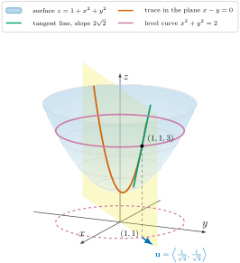
The surface \(z = 1 + x^2 + y^2\text{,}\) an upward-opening paraboloid, drawn as a translucent blue surface. A translucent yellow vertical plane \(x - y = 0\) passes through the surface above the line \(y = x\) in the \(xy\)-plane, where the unit vector \(\mathbf u\) is drawn as a blue arrow starting at \((1,1,0)\text{.}\) The plane meets the surface in a parabola, drawn in solid vermillion, and a green tangent line touches this parabola at the marked point \((1,1,3)\text{.}\) The slope of this tangent line, measured within the vertical plane, is the directional derivative \(2\sqrt 2\text{.}\) A reddish-purple circle on the surface at height \(z = 3\) marks the level curve \(f = 3\text{,}\) and its dashed projection in the \(xy\)-plane is the circle \(x^2 + y^2 = 2\) through the point \((1,1)\text{.}\)
Instructions.
Drag the slider to rotate the direction \(\mathbf u = \langle\cos\varphi, \sin\varphi\rangle\) at the point \((1,1)\text{.}\) The vertical plane through \((1,1)\) in the direction \(\mathbf u\) cuts the surface \(z = 1 + x^2 + y^2\) in a curve, and the tangent line to this curve at \((1,1,3)\) has slope \(D_{\mathbf u} f = \left(\nabla f\right)_{(1,1)}\cdot\mathbf u\text{,}\) displayed above the figure. Use the buttons to snap \(\mathbf u\) to the direction of \(\nabla f\text{,}\) its opposite, or a direction of zero change. Drag the figure to view it from a different angle, or press the “Rotate” button to spin it automatically.

