Finally, we are in a position to define the two important trigonometric functions \(f(t) = \sin(t)\) and \(g(t) = \cos(t)\text{.}\) We will use the trigonometric ratios \(\sin(\alpha)\) and \(\cos(\alpha)\) to define values of the functions at any given \(t\text{,}\) although in applications the functions are often detached from their unit circle meaning. Here is the definition.
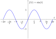
What is the graph of the sine function \(f(t) = \sin(t)\text{?}\) We know that for the angle of \(t\) radians in standard position, \(\sin(t)\) is the \(y\) coordinate of the point \(P = (x, y)\) at which the terminal side intersects the unit circle, as shown in Figure 8.3.1. We start from \(t = 0\) and examine how the \(y\) coordinate of the point of intersection changes as \(t\) increases.
At \(t = 0\) the terminal side of the angle 0 radians coincides with the initial side; the point of intersection is \(P = (x, y) = (1, 0)\text{.}\) Hence, \(y = 0\) and \(\sin(0) = 0\text{.}\) Continuing to increase \(t\text{,}\) then for an angle whose terminal side is in the first quadrant, the \(y\) coordinate is between \(0\) and \(1\text{,}\) and it increases as \(t\) increases. When the angle \(t\) reaches \(\frac{\pi}{2} = 90^{\circ}\text{,}\) the terminal side is vertical, the point of intersection with the unit circle is \(P = (0, 1)\text{;}\) the \(y\) coordinate is \(y = 1\text{.}\) That is, \(\sin(\frac{\pi}{2}) = 1\text{.}\) Look at the graph in Figure 8.4.2. For \(t\) between \(0\) and \(\frac{\pi}{2}\) the function \(\sin(t)\) increases from \(0\) to \(1\text{.}\) Past \(t = \frac{\pi}{2}\text{,}\)\(\sin(t)\) decreases when \(t\) increases until it hits \(0\) at \(t = \pi\text{.}\)
If we keep increasing \(t\) past \(\frac{\pi}{2}\text{,}\) the terminal side is in the second quadrant and the \(y\) coordinate is now decreasing until it is \(0\) at \(t = \pi = 180^{\circ}\text{.}\) Continuing to increase \(t\) past \(\pi\text{,}\) the terminal side is now in the third quadrant. The \(y\) coordinate is now negative and is getting “more and more negative” until it hits \(-1\) at \(\frac{3\pi}{2}\text{.}\) Note how the graph of \(\sin(t)\) in Figure 8.4.2 reflects this behavior. When the terminal side of the angle \(t\) is in the fourth quadrant the \(y\) coordinate is getting “less and less negative” when \(t\) increases until at \(t = 2\pi = 360^{\circ}\) the terminal side is aligned again with the positive \(x\)-axis with \(y = 0\text{.}\) If we keep increasing \(t\) past \(2\pi\) the same cycle of changes in \(y\) repeats on the interval \(2\pi \lt t \lt 4\pi\text{.}\) Therefore, the values of \(\sin(t)\) repeat for \(2\pi \lt t \lt 4\pi\text{.}\) And so on.
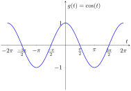
To obtain the graph of the function \(\cos(t)\text{,}\) we follow changes in the \(x\)-coordinate of the intersection point \(P = (x, y)\) as the angle \(t\) changes. We easily obtain the graph of \(g(t) = \cos(t)\) given in Figure 8.4.3.
As we see from the definition and from the graphs of the sine and cosine functions, both functions \(\sin(t)\) and \(\cos(t)\) are periodic with period \(2\pi\text{:}\)
The amplitude of both functions is \(1\text{,}\) the equilibrium is \(0\text{,}\) and the midline is the \(x\)-axis (\(y=0\)). This can be verified by observing that
Indeed, if angle \(t\) changes sign, the \(y\) coordinate of the intersection point of its terminal side with the unit circle changes sign while the \(x\) coordinate stays the same.
You can use your graphing calculator to graph the sine and cosine functions, but you have to remember to set your calculator in radians and not in degrees. The values \(\sin(t)\) and \(\cos(t)\) were defined by interpreting \(t\) as an angle in radians.
SubsectionTransforming Sine and Cosine Functions—Basic Ideas
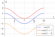
It took a lot of work to define the sine and cosine functions. The good news is that once we have them, they are easy to use. All that we usually need to remember are the graphs of the functions \(y = \sin(t)\) and \(y = \cos(t)\) as given in Figure 8.4.2 and Figure 8.4.3.
Speaking of graphs, notice that the function \(\cos(t)\) starts from its maximum value at \(t = 0\text{,}\)\(\cos(0) = 1\text{.}\) The sine function on the other hand starts at \(t = 0\) from its equilibrium value, \(\sin(0) = 0\text{.}\) These observations will be important in the next section when we try to match given periodic functions with a transformed sine or cosine function.
We used the unit circle and interpreted \(t\) as an angle to define the sine and cosine functions. In applications, we will typically get away from this interpretation. The independent variable \(t\) will most often be time, and we will use the sine and cosine functions as convenient periodic functions that are useful for modeling periodic processes. We will use the notation \(y = \sin(t)\) and \(y = \cos(t)\) where \(y\) denotes the dependent variable and is no longer related to coordinates on the unit circle.
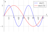
The sine and cosine functions, \(y = \sin(t)\) and \(y = \cos(t)\text{,}\) wouldn’t be very useful for modeling real-life periodic processes if we couldn’t transform them to change the period, amplitude, or midline. How many real-life periodic processes have the period of exactly \(2\pi\text{,}\) amplitude \(1\text{,}\) and equilibrium \(0\text{?}\) Not many. Fortunately, we can easily change all three numbers by vertical scaling and shifting and horizontal scaling.
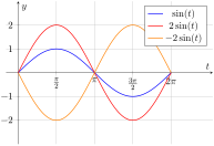
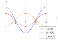
We learned in the previous chapter that multiplying the output by a constant corresponds to vertical scaling of the graph. Here are the graphs of the functions in parts 1 and 2 and the original function \(y = \sin(t)\) in one coordinate system:
The amplitude of both \(y = 2\sin(t)\) and \(y = -2\sin(t)\) is \(2\text{,}\) the period is \(2\pi\text{,}\) and the midline is \(y = 0\text{.}\) Recall that vertical scaling changes the amplitude only. If we multiply by a negative constant, we additionally have the reflection of the scaled graph over the \(t\)-axis.
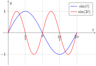
From the graph, it is evident that the function \(y = \sin(2t)\) executes a full cycle from \(t=0\) to \(t=\pi\text{.}\) Hence, the period of \(y = \sin(2t)\) is \(\pi\text{.}\) The amplitude of the function is still \(1\) and the midline \(y = 0\text{.}\)
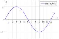
Suppose that we want a periodic function with a period \(12\text{.}\) Indeed, the first periodic function considered in this chapter had period \(12\text{.}\) Can we find such a function? Yes. Soon we will learn a systematic technique for doing this; for now, here is an example.
Now that we have seen how to manipulate the sine and cosine functions to change the period, amplitude, and midline, our next step is to combine these transformations to change all three quantities.
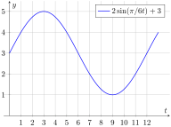
What is the period, amplitude, and midline of the function \(p(t)\text{?}\) What transformations have been applied to \(\sin(t)\) to obtain \(p(t)\text{?}\)
Clearly we are looking at one cycle of a transformed sine function, so the period is \(12\text{.}\) Since \(p_\text{max} = 5\text{,}\)\(p_\text{min} = 1\text{,}\) the amplitude is \(2\) and the midline is \(y = 3\text{.}\)
We applied horizontal scaling by the factor of \(\frac{\pi}{6}\text{,}\) vertical scaling by the factor of \(2\text{,}\) and a vertical shift by \(3\text{.}\)
For each of the following, use a graph to identify the period, amplitude, and midline of the given function. Identify what transformations have been applied to either \(f(t)=\cos(t)\) or \(f(t)=\sin(t)\) to obtain the given function.
period: \(2\pi\text{;}\) amplitude: \(5\text{;}\) midline: \(y=0\text{.}\)\(y\) is the graph of \(f(t)=\cos(t)\) stretched vertically by a factor of \(5\)
period: \(2\pi\text{;}\) amplitude: \(4\text{;}\) midline: \(y=0\text{.}\)\(y\) is the graph of \(f(t)=\sin(t)\) stretched vertically by a factor of \(4\) and reflected over the \(t\)-axis
period \(\frac{2\pi}{5}\text{;}\) amplitude: \(1\text{;}\) midline: \(y=0\text{.}\)\(y\) is the graph of \(f(t)=\sin(t)\) compressed horizontally by a factor of \(5\)
period: \(6\text{;}\) amplitude: \(1\text{;}\) midline: \(y=0\text{.}\)\(y\) is the graph of \(f(t)=\cos(t)\) compressed horizontally by a factor of \(\pi\) and stretched horizontally by a factor of \(3\)
period: \(\frac{10\pi}{3}\text{;}\) amplitude: \(1\text{;}\) midline: \(y=0\text{.}\)\(y\) is the graph of \(f(t)=\sin(t)\) compressed horizontally by a factor of \(3\) and stretched horizontally by a factor of \(5\)
period: \(2\pi\text{;}\) amplitude: \(2\text{;}\) midline: \(y=-6\text{.}\)\(y\) is the graph of \(f(t)=\cos(t)\) stretched vertically by a factor of \(2\) and shifted down \(6\) units
period: \(\pi\text{;}\) amplitude: \(3\text{;}\) midline: \(y=0\text{.}\)\(y\) is the graph of \(f(t)=\sin(t)\) compressed horizontally by a factor of \(2\text{,}\) stretched vertically by a factor of \(3\text{,}\) and reflected over the \(t\)-axis
period: \(4\text{;}\) amplitude: \(10\text{;}\) midline: \(y=4\text{.}\)\(y\) is the graph of \(f(t)=\sin(t)\) compressed horizontally by a factor of \(\pi\text{,}\) stretched horizontally by a factor of \(2\text{,}\) stretched vertically by a factor of \(10\text{,}\) and shifted up \(4\) units