Section 5.2 Graphs of Exponential Functions

In the previous section we looked at algebraic properties of exponential functions and applied examples involving exponential functions. In this section we study graphs of exponential functions.
The graph of an exponential function \(f(t) = A \cdot b^t\) depends on whether the growth factor \(b\) is greater than \(1\) or less than \(1\text{.}\)

Example 5.2.1.

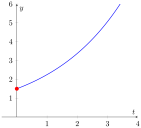
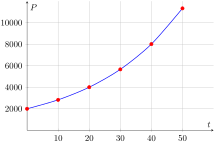
Graph the function of ExampleΒ 5.1.3 that describes the population \(P\) of E. coli bacteria in a laboratory culture \(t\) minutes after the experiment began:
\begin{equation*} P = f(t) = 2000(1.0353)^t. \end{equation*}
The table of values for \(t\) taken every \(10\) minutes is as follows:
\(t\) (minutes) \(0\) \(10\) \(20\) \(30\) \(40\) \(50\)
\(P\) (\(\#\) of bacteria) \(2000\) \(2829.4\) \(4002.7\) \(5662.6\) \(8010.8\) \(11332.9\)
The graph reflecting the data is:
The function increases, and increasingly fast: the population of E. coli bacteria grows faster and faster over time.
Observe that we drew the graph only for \(t \geq 0\) as the experiment begins at \(t = 0\text{,}\) even though the function \(P = 2000(1.0353)^t\) is defined for all \(t\text{.}\)

Example 5.2.2.

Graph the function
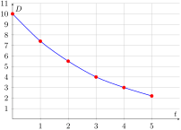
\begin{equation*} D(t) = 10(0.74)^t \end{equation*}
that shows the amount of Diazepam, in mg, left in the body \(t\) days after a single \(10\) mg dose.
Since the growth factor \(0.74\) is less than \(1\text{,}\) \(D(t)\) is a decreasing function. Here are the values of \(D(t)\) for \(t = 0, 1, 2, 3, 4, 5\) along with the corresponding graph:
\(t\) (days) \(0\) \(1\) \(2\) \(3\) \(4\) \(5\)
\(D\) (mg) \(10\) \(7.4\) \(5.5\) \(4.0\) \(3.0\) \(2.2\)
The amount by which the function is decreasing daily is less and less as time goes on. The function decreases daily by \(26\%\) of the current amount, so the smaller the current amount the smaller the decrease.
In general, the shape of the graph of an exponential function \(y = A \cdot b^x\) is different for the base \(b \gt 1\) and for \(b \lt 1\text{:}\)

Instructions.

Change the values of \(A\) and \(b\) to see how \(f(x) = A \cdot b^x\) changes.
Figure 5.2.3.
If \(b \gt 1\text{,}\) the function \(f(t) = A \cdot b^t\) is increasingβ€”its graph is climbing as it is traced from left to right. If \(b \lt 1\text{,}\) the function \(f(t) = A \cdot b^t\) is decreasingβ€”its graph is falling as it is traced from left to right. In both cases the values of \(y = A \cdot b^x\) are always positive, so the graph is entirely above the \(x\)-axis. The \(y\)-intercept is always equal to the initial value \(A\text{.}\)

Example 5.2.4.

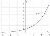
Graph the function \(y=2^x\)
The initial value is \(A = 1\) and the growth factor (base) is \(b = 2\text{.}\) Since \(b\) is greater than \(1\text{,}\) the graph is increasing:
Note that for \(x \gt 0\text{,}\) \(2^x \gt 1\) and \(2^x\) increases as \(x\) increases:
\begin{equation*} 2^1 = 2, \quad 2^2 = 4, \quad 2^3 = 8, \quad 2^4 = 16, \quad \dots \end{equation*}
For \(x \lt 0\text{,}\) \(2^x \lt 1\) and \(2^x\) becomes smaller and smaller as \(x\) becomes β€œmore and more negative”:
\begin{equation*} 2^{-1} = \dfrac{1}{2}, \quad 2^{-2} = \dfrac{1}{2^2} = \dfrac{1}{4}, \quad 2^{-3} = \dfrac{1}{2^3} = \dfrac{1}{8}, \quad 2^{-4} = \dfrac{1}{2^4} = \dfrac{1}{16}, \quad \dots \end{equation*}
In fact, as \(x\) becomes β€œmore and more negative”, \(2^x\) becomes arbitrarily close to \(0\) without ever reaching itβ€”the graph approaches the \(x\)-axis but never crosses it. We say that the \(x\)-axis is a horizontal asymptote of the function \(y = 2^x\text{.}\)

Example 5.2.5.

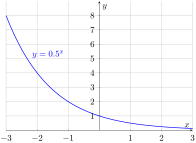
Graph the function \(y = \left(\dfrac{1}{2}\right)^x\text{.}\)
Note that once again \(A = 1\) but, in contrast to the last example, the growth factor \(b = \frac{1}{2} = 0.5\text{.}\) As \(b \lt 1\text{,}\) the graph is decreasing:
Observe that \(\left(\dfrac{1}{2}\right)^x \lt 1\) for \(x \gt 0\text{,}\) and \((\dfrac{1}{2})^x\) decreases as \(x\) increases:
\begin{equation*} \left( \dfrac{1}{2} \right)^1 = \dfrac{1}{2}, \quad \left( \dfrac{1}{2} \right)^2 = \dfrac{1}{4}, \quad \left( \dfrac{1}{2} \right)^3 = \dfrac{1}{8}, \quad \dots \end{equation*}
This means the \(x\)-axis is a horizontal asymptote of the function \((\frac{1}{2})^x\text{.}\)
On the other side, as \(x\) becomes β€œmore and more negative”, \(\left(\dfrac{1}{2}\right)^x\) becomes larger and larger:
\begin{equation*} \left( \dfrac{1}{2} \right)^{-1} = \dfrac{1}{\frac{1}{2}} = 2, \quad \left( \dfrac{1}{2} \right)^{-2} = \dfrac{1}{(\frac{1}{2})^2} = \dfrac{1}{\frac{1}{4}} = 4, \quad \left( \dfrac{1}{2} \right)^{-3} = \dfrac{1}{(\frac{1}{2})^3} = \dfrac{1}{\frac{1}{8}} = 8, \quad \dots \end{equation*}

Example 5.2.6.

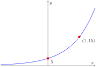
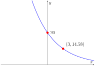
For each graph shown below, find the formula for the function in the form \(f(x) = A \cdot b^x\text{:}\)
Solution.
We have to find the initial value \(A\) and the growth factor \(b\text{.}\) Since \(A\) is always the \(y\)-intercept, we have \(A = 5\) and so \(f(x) = 5 \cdot b^x\text{.}\) To find \(b\text{,}\) note that the point \((1, 15)\) is on the graph so the equation \(f(1) = 5 \cdot b^1 = 5 \cdot b = 15\) must hold. That is, \(5 \cdot b = 15\) which gives \(b = 3\text{.}\) Thus, the function corresponding to the graph (a) is \(f(x) = 5 \cdot 3^x\text{.}\)
In the second graph, the initial value is \(A = 20\text{.}\) By using the point \((3, 14.58)\text{,}\) we can set up an equation to solve for \(b\text{:}\)
\begin{align*} f(3) \amp = 14.58\\ 20 \cdot b^3 \amp = 14.58\\ b^3 \amp = 14.58 / 20\\ b \amp = (0.729)^{1/3}\\ b \amp = 0.90 \end{align*}
This means \(f(x) = 20 \cdot 0.90^x\text{.}\)

Example 5.2.7.

Find a function \(f(t) = A \cdot b^t\) whose graph contains points \((1, 15)\) and \((2, 22.5)\text{.}\)
Solution.
Observe that neither given point is the vertical intercept of the function, soβ€”unlike the last examplesβ€”we do not immediately have \(A\text{.}\) Our starting point is recognizing that \((1, 15)\) is on the graph of \(f(t)\) and so \(f(1) = 15\text{.}\) Similarly, \((2, 22.5)\) implies \(f(2) = 22.5\text{.}\) Therefore, the following two equations must hold:
\begin{equation*} A \cdot b^1 = 15 \quad \text{and} \quad A \cdot b^2 = 22.5. \end{equation*}
To find \(A\) and \(b\text{,}\) we can divide these two equations to obtain
\begin{align*} \frac{A \cdot b^2}{A \cdot b^1} \amp = \dfrac{22.5}{15}\\ \dfrac{b^2}{b} \amp = \dfrac{22.5}{15}\\ b \amp = 1.5 \end{align*}
Now we know that \(f(t) = A \cdot 1.5^t\text{,}\) but \(A\) is still unknown. Using either of the given point on the graph, we can solve for \(A\text{.}\) Suppose we choose to use \(f(1) = 15\)β€”then \(A \cdot 1.5^1 = 15\) which gives \(A = \frac{15}{1.5} = 10\text{.}\) Thus, \(f(t) = 10(1.5)^t\text{.}\)
Exercises Exercises

1.

Complete the table of values below and use it to graph the exponential function \(\displaystyle y=3^x\) in the interval \(-3\leq x \leq 3\text{.}\)
\(x\) \(-3\) \(-2\) \(-1\) \(0\) \(1\) \(2\) \(3\)
\(y=3^x\) \(\frac{1}{27}\) \(?\) \(?\) \(?\) \(?\) \(?\) \(?\)
Solution.
\(x\) \(-3\) \(-2\) \(-1\) \(0\) \(1\) \(2\) \(3\)
\(y=3^x\) \(\frac{1}{27}\) \(\frac{1}{9}\) \(\frac{1}{3}\) \(1\) \(3\) \(9\) \(27\)

2.

Complete the table of values below and use it to graph the exponential function \(\displaystyle y=\left(\frac{1}{3}\right)^x\) in the interval \(-3\leq x \leq 3\text{.}\)
\(x\) \(-3\) \(-2\) \(-1\) \(0\) \(1\) \(2\) \(3\)
\(y=\left(\frac{1}{3}\right)^x\) \(27\) \(?\) \(?\) \(?\) \(?\) \(?\) \(?\)
Solution.
\(x\) \(-3\) \(-2\) \(-1\) \(0\) \(1\) \(2\) \(3\)
\(y=\left(\frac{1}{3}\right)^x\) \(27\) \(9\) \(3\) \(1\) \(\frac{1}{3}\) \(\frac{1}{9}\) \(\frac{1}{27}\)

3.

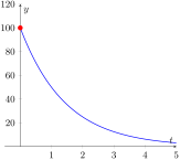
Below you see a graph of an exponential function \(y=A\cdot b^t\text{.}\) What is its initial value \(A\text{?}\) Is its growth factor \(b\) greater than \(1\) or less than \(1\text{?}\)
Solution.
\(A=100\text{;}\) \(b\lt 1\)

4.

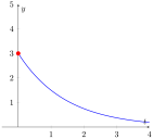
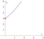
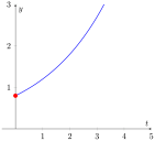
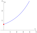
Which of the graphs below could be a graph of the function \(y=3(1.5)^t\text{?}\) Explain your answer!

5.

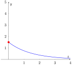
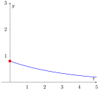
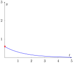
Which of the graphs below could be a graph of the function \(y=0.8(0.75)^t\text{?}\) Explain your answer!

6.

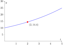
Find a formula in the form \(y=A\cdot b^t\) for the exponential function whose graph is given below:
Solution.
\(y=10(1.2)^t\)

7.

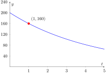
Find a formula in the form \(y=A\cdot b^t\) for the exponential function whose graph is given below:
Solution.
\(y=200(0.8)^t\)

8.

Find a function \(f(x)=A\cdot b^x\) whose graph contains points \((0,500)\) and \((4,120.05)\text{.}\)
Solution.
\(y=500(0.7)^x\)

9.

Find a function \(g(x)=A\cdot b^x\) whose graph contains points \((1,48)\) and \((2,76.8)\text{.}\)
Solution.
\(y=30(1.6)^x\)

10.

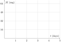
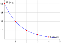
A medication is eliminated from the body at the daily percent rate of \(50\%\text{.}\) A patient takes a single dose of \(64\) mg of the medication. Let \(M(t)\) be the amount, in mg, remaining in the patient’s body \(t\) days after the dose.

(b)

Fill in the missing entries in the following table of values:
\(t\) (days) \(0\) \(1\) \(2\) \(3\) \(4\)
\(M(t)\) mg \(?\) \(?\) \(?\) \(?\) \(?\)
Solution.
\(t\) (days) \(0\) \(1\) \(2\) \(3\) \(4\)
\(M(t)\) mg \(64\) \(32\) \(16\) \(8\) \(4\)

(c)

Use the table to plot the points corresponding to \(t=0,1,2,3,4\) that are on the graph of \(M(t)\text{.}\) Sketch a graph of the function \(M=M(t)\) in the coordinate system below.
Solution.

11.

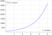
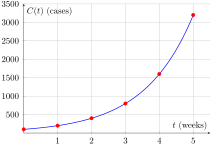
The number of diagnosed cases of a new virus doubles every week. Let \(C(t)\) be the number of diagnosed cases \(t\) weeks after an epidemic began. Here are the measurements during the first weeks:
\(t\) (weeks) \(0\) \(1\) \(2\) \(3\) \(4\) \(5\)
\(C(t)\) (cases) \(100\) \(200\) \(400\) \(800\) \(1600\) \(3200\)

(a)

Mark the points corresponding to the data in the table on the graph of the function \(C(t)\text{:}\)
Solution.

(b)

Is the function \(C=C(t)\) exponential? If yes, find a formula for \(C(t)\) and check with the table of values.
Solution.
Yes; \(C(t)=100(2)^t\)
You have attempted of activities on this page.